How To Insert Multiple Rows In Excel

Methods to Insert Multiple Rows in Excel

Microsoft Excel is a powerful tool for organizing and analyzing data. When working with large data sets or creating complex spreadsheets, it often becomes necessary to insert multiple rows to accommodate new information. Thankfully, Excel offers several methods to accomplish this task efficiently. In this article, we will explore ten different ways to insert multiple rows in Excel.

Method 1: Using the Insert Command: The easiest way to insert multiple rows in Excel is by using the Insert command. Simply select the desired number of rows, right-click, and choose Insert from the context menu.

Method 2: Using the Ctrl Key: Hold the Ctrl key while selecting multiple rows, right-click, and choose Insert from the context menu. This method is useful when you need to insert consecutive rows.

Method 3: Using the Right-Click Menu: Right-click on a selected row or rows, choose Insert, and select either “Insert Rows Above” or “Insert Rows Below” from the drop-down menu.

Method 4: Using the Ribbon Menu: Go to the Home tab in the Excel ribbon, click on the Insert dropdown, and choose “Insert Sheet Rows” to insert multiple rows at once.

Method 5: Using a Keyboard Shortcut: Press Shift + Spacebar to select the entire row, then press Ctrl + Shift + “+” (plus sign) to insert multiple rows above the selected row.

Method 6: Inserting Rows Based on a Pattern or Formula: If you need to insert rows based on a pattern or formula, you can use Excel’s built-in features such as the Fill Handle or Insert Function.

Method 7: Using the TRANSPOSE Function: If you have data arranged horizontally and want to convert it to a vertical format, you can use the TRANSPOSE function to insert multiple rows and transpose the data.

Method 8: Inserting Multiple Rows in a Specific Location: To insert multiple rows in a specific location within a worksheet, select the desired number of rows, right-click, and choose “Insert Copied Cells.” This method is useful when you want to maintain a specific order of data.

Method 9: Inserting Rows in a Filtered Worksheet: If your worksheet is filtered, you can insert rows in the visible filtered range by selecting the desired number of rows, right-clicking, and choosing “Insert” from the context menu.

Method 10: Applying the Same Row Insertion to Multiple Worksheets: If you have multiple worksheets within a workbook and need to insert rows in the same location on all worksheets, you can group the worksheets and apply the row insertion on all sheets simultaneously.

By utilizing these methods, you can easily insert multiple rows in Excel based on your specific requirements. Experiment with these techniques and choose the one that best suits your needs, saving time and ensuring data integrity within your spreadsheets.

Method 1: Using the Insert command

One of the easiest ways to insert multiple rows in Excel is by using the Insert command. This method allows you to quickly add rows above or below the selected row or rows.

To use this method, follow these steps:

1. Select the row or rows where you want to insert new rows. You can do this by clicking on the row number or by using the Shift key to select multiple rows.
2. Right-click anywhere within the selected rows to open the context menu. Alternatively, you can go to the Home tab in the Excel ribbon and click on the Insert dropdown.
3. In the context menu or the Insert dropdown, choose “Insert” to open the Insert dialog box.
4. In the Insert dialog box, select “Entire row” and click on the OK button.

Excel will insert the specified number of rows above or below the selected rows, moving the existing rows down.

This method is particularly useful when you need to insert multiple rows at once and want to maintain the order of your data. It is a straightforward and efficient way to add rows to your spreadsheet without disrupting the existing content.

For example, let’s say you have a sales spreadsheet with data for different products. If you want to add new rows for additional products, you can easily select the last row of the existing data, use the Insert command to insert multiple rows below it, and then populate the new rows with the details of the new products.

By using the Insert command, you can quickly expand your spreadsheet, accommodate new information, and maintain the organization of your data. This method is ideal for situations where you need to insert rows without rearranging the existing content.

Method 2: Using the Ctrl key

Another convenient method for inserting multiple rows in Excel is by using the Ctrl key. This method is particularly useful when you want to insert consecutive rows quickly.

To use this method, follow these steps:

1. Select the first row from where you want to begin inserting new rows.
2. Hold down the Ctrl key on your keyboard.
3. While holding the Ctrl key, use the arrow key (up or down) to select the number of rows you want to insert.
4. Once the desired number of rows is selected, right-click anywhere within the selected rows to open the context menu.
5. In the context menu, choose “Insert” to insert new rows above the selected rows.

By using the Ctrl key, you can quickly select multiple consecutive rows without having to click on each individual row. This method saves time and allows for a seamless row insertion process.

For example, let’s say you have a table where you want to insert five new rows between rows 6 and 7. Instead of manually selecting each row in between, you can simply select the first row (row 6) and hold the Ctrl key while using the down arrow key to select the next five rows. Then, right-click and choose “Insert” to insert the new rows above the selected rows.

The Ctrl key method is a great way to insert multiple consecutive rows quickly and efficiently. It eliminates the need for manual row selections and streamlines the process of adding new rows to your spreadsheet.

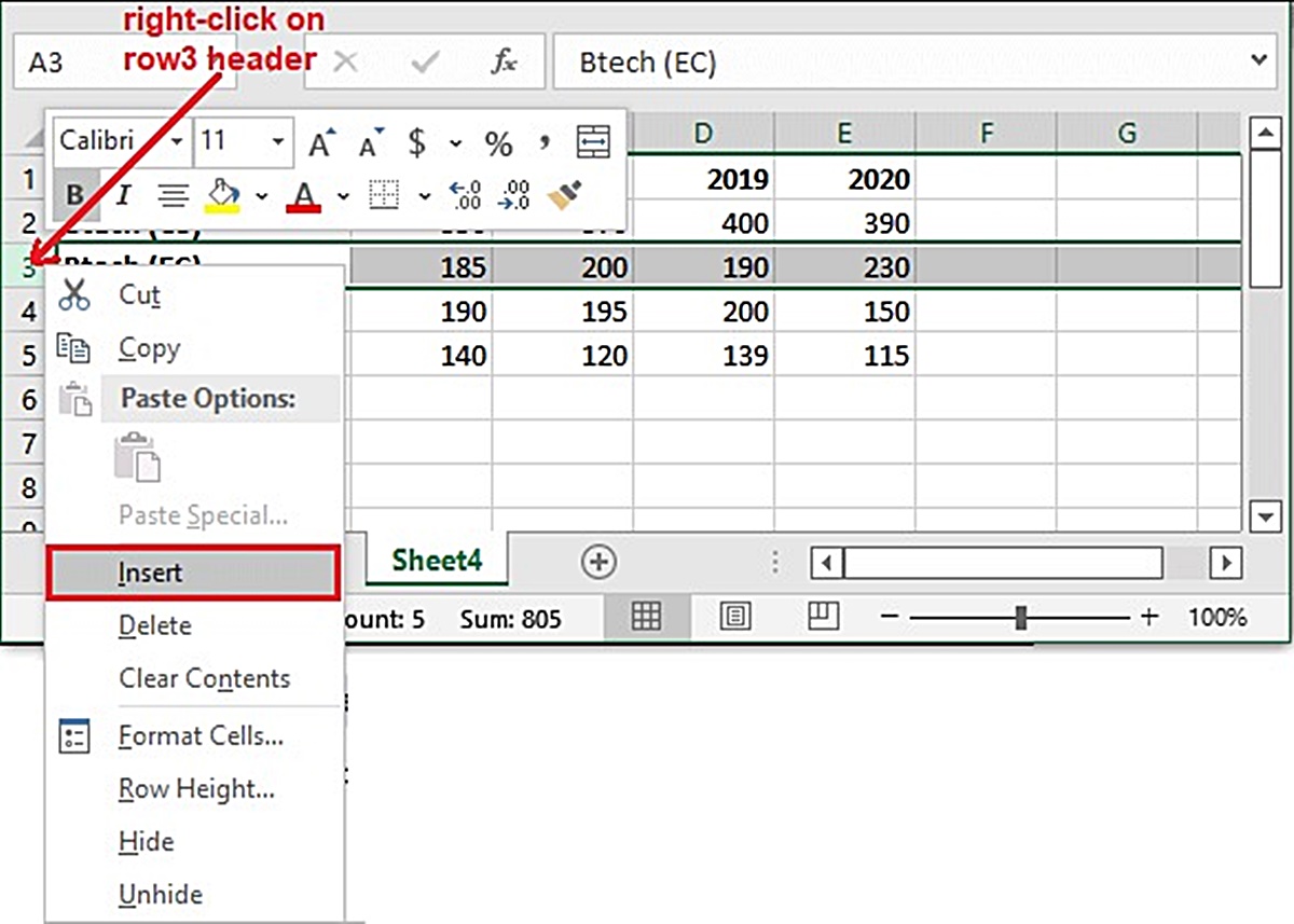
Method 3: Using the right-click menu

If you prefer a more straightforward approach to insert multiple rows in Excel, you can utilize the right-click menu. This method allows you to easily add new rows above or below the selected row or rows.

To use this method, follow these steps:

1. Select the row or rows where you want to insert new rows. You can do this by clicking on the row number or by using the Shift key to select multiple rows.
2. Right-click anywhere within the selected rows to open the context menu.
3. In the context menu, choose “Insert” to expand the sub-menu options.
4. In the sub-menu options, select either “Insert Rows Above” or “Insert Rows Below” depending on where you want the new rows to be inserted.

Excel will insert the specified number of rows above or below the selected rows, pushing the existing rows down accordingly.

This method is convenient and intuitive, allowing you to easily add rows to your spreadsheet as needed. By using the right-click menu, you can quickly insert multiple rows without the need to navigate through various menu options.

For example, suppose you have a budget worksheet where you want to add new rows for additional expenses. By selecting the last row of your current data and using the right-click menu to insert rows below, you can easily create space to enter the new expenses while keeping the rest of the budget intact.

Using the right-click menu method provides a simple and efficient way to insert multiple rows in Excel, ensuring that your data remains organized and structured.

Method 4: Using the Ribbon menu

If you prefer using the Excel Ribbon menu for executing commands, you can also insert multiple rows using this method. The Ribbon menu provides a visual and accessible way to perform various actions in Excel, including adding new rows.

To use this method, follow these steps:

1. Open your Excel spreadsheet and navigate to the worksheet where you want to insert rows.
2. Go to the Home tab in the Excel Ribbon located at the top of the Excel window.
3. In the Home tab, locate the Insert dropdown in the Cells group.
4. Click on the Insert dropdown to expand the menu options.
5. In the expanded menu options, select “Insert Sheet Rows”.

By choosing “Insert Sheet Rows” from the Ribbon menu, Excel will insert new rows above the currently selected row, pushing the existing rows downwards.

This method is ideal for users who prefer using the Excel Ribbon and want a visual representation of the available commands. It provides a straightforward way to insert multiple rows without having to navigate through various menus and submenus.

For example, let’s say you have a sales tracker where you want to add new rows to accommodate additional sales data. By selecting the appropriate location and using the Ribbon menu to insert sheet rows, you can easily make room for the new information without disrupting the existing data.

Using the Ribbon menu method to insert multiple rows in Excel allows for a seamless and user-friendly experience, ensuring that you can efficiently manage your spreadsheet without any hassle.

Method 5: Using a keyboard shortcut

If you prefer using keyboard shortcuts to perform actions in Excel, you can take advantage of a specific shortcut to quickly insert multiple rows in your spreadsheet. This method allows for a fast and efficient way to add rows without the need to navigate through menus or use the mouse.

To use this method, follow these steps:

1. Select the entire row that you want to insert new rows above or below. To select the entire row, press the Shift key and the Spacebar simultaneously.
2. With the entire row selected, press the Ctrl, Shift, and Plus(+) keys together. The Plus(+) key is usually located on the numeric keypad section of the keyboard.

Upon pressing the Ctrl, Shift, and Plus(+) keys, Excel will insert a new row or rows above the selected row, pushing the existing rows downward.

This keyboard shortcut method is beneficial for users who prefer a more efficient and hands-on approach to Excel tasks. It enables you to quickly insert multiple rows without interrupting your workflow or relying on the mouse for commands.

For example, let’s say you have a project plan where you want to add ten new rows above the current row. By selecting the desired row, such as the last row of completed tasks, and using the keyboard shortcut, you can swiftly create space for the upcoming tasks.

Using the keyboard shortcut method to insert multiple rows in Excel is a time-saving technique, allowing you to stay focused on your keyboard-centered workflow while efficiently expanding your spreadsheet.

Method 6: Inserting rows based on a pattern or formula

In Excel, you have the option to insert rows based on a specific pattern or formula. This method is particularly useful when you need to insert rows that follow a certain sequence or when you want to automate the process using a formula.

To use this method, follow these steps:

1. Determine the pattern or formula that you want to apply to the new rows.
2. Select the existing row or rows that contain the pattern or formula you want to replicate.
3. Right-click on the selected row(s) and choose “Insert” from the context menu.
4. Excel will insert new rows above the selected row(s) and copy the pattern or formula to the newly inserted rows.

This method allows you to insert multiple rows at once while adhering to a specific pattern or formula. It can be highly beneficial when you have a predefined sequence or need to calculate values based on existing data.

For example, let’s say you have a table with a formula in the first row that calculates the total cost based on the quantity and unit price. If you need to insert ten additional rows with the same formula, you can select the existing row, right-click, and choose “Insert” to add the new rows while automatically copying the formula to each inserted row.

By utilizing this method, you can save time and effort by avoiding the manual entry or copy-pasting of patterns or formulas. Excel will handle the duplication of the pattern or formula, ensuring that the new rows match the desired sequence or calculation.

Method 7: Using the TRANSPOSE function

The TRANSPOSE function in Excel allows you to convert data arranged horizontally into a vertical format and vice versa. By utilizing this function, you can also insert multiple rows in Excel. This method is beneficial when you need to rearrange data and create additional rows in the process.

To use this method, follow these steps:

1. Select the range of cells that you want to transpose and insert as rows.
2. Copy the selected range by pressing Ctrl+C on your keyboard.
3. Select the cell where you want to insert the transposed data in a new location.
4. Right-click on the selected cell and choose “Paste Special” from the context menu.
5. In the Paste Special dialog box, check the “Transpose” option.
6. Click on the OK button to insert the transposed data as rows.

Excel will insert multiple rows based on the size of the pasted range and arrange the data vertically, creating a new row for each original column in the transposed range.

This method is particularly useful when you have data that needs to be rearranged vertically or when you want to insert rows based on the number of columns in the transposed range.

For instance, if you have data arranged in columns and want to insert multiple rows for each column, you can use the TRANSPOSE function to convert the data into rows. This allows you to create new rows while maintaining the integrity of the original information.

By utilizing the TRANSPOSE function, you can easily insert multiple rows in Excel while reorganizing your data to best fit your needs.

Method 8: Inserting multiple rows in a specific location

When working with complex Excel spreadsheets, you may need to insert multiple rows in a specific location rather than at the beginning or end of the data. Excel provides a method to insert rows at a precise location within your worksheet, allowing you to maintain the specific order of your data.

To use this method, follow these steps:

1. Select the row or rows below which you want to insert new rows. You can do this by clicking on the row number or by using the Shift key to select multiple rows.
2. Right-click anywhere within the selected rows to open the context menu.
3. In the context menu, choose “Insert Copied Cells” to open the Insert Copied Cells dialog box.
4. In the dialog box, select “Shift Cells Down” and click on the OK button.

By using this method, Excel will insert the specified number of rows above the selected rows, shifting the existing rows downward accordingly.

This method is extremely useful when you have a specific location within your dataset where you need to insert new rows. It ensures that the order of your data remains intact and that the newly inserted rows are correctly positioned.

For example, let’s say you have a sales report with various sections, and you want to add new rows between two specific sections. By selecting the last row of the upper section and using the “Insert Copied Cells” method, you can insert the necessary rows in the desired location, keeping the sections separate and organized.

Using the “Insert Copied Cells” method allows you to insert multiple rows at a specific location within your Excel worksheet, ensuring that your data is accurately placed according to your needs.

Method 9: Inserting rows in a filtered worksheet

When working with a filtered worksheet in Excel, you might need to insert rows within the filtered range rather than inserting rows outside of the filtered data. Excel offers a method that allows you to insert multiple rows while accounting for the applied filter, ensuring that the newly inserted rows belong to the visible filtered range.

To use this method, follow these steps:

1. Apply a filter to your worksheet by selecting the data range and going to the Data tab in the Excel Ribbon. Click on the Filter button to enable filtering.
2. Filter the data based on the specified criteria to display the desired subset of the data.
3. Select the row or rows within the filtered range where you want to insert new rows. You can do this by clicking on the row number or by using the Shift key to select multiple rows.
4. Right-click anywhere within the selected rows to open the context menu.
5. In the context menu, choose “Insert” to insert new rows above the selected rows. The insertion will be confined within the visible filtered range.

By using this method, Excel will insert the specified number of rows above the selected rows, while ensuring that the newly inserted rows are part of the filtered range and not affecting the hidden rows.

This method is particularly useful when you need to insert rows within a filtered dataset, such as adding new entries to a filtered sales report without disrupting the visibility of other filtered data.

For example, let’s say you have a table with sales data for multiple regions, and you want to insert new rows to include additional sales figures for a specific region. By filtering the data for that region, selecting the appropriate location, and using the “Insert” method, you can insert rows within the filtered range, adding the desired information without affecting the visibility of other regions in the filtered view.

Using the “Insert” method in a filtered worksheet allows you to insert multiple rows precisely where you need them within the filtered range, providing a seamless way to update your data without compromising the visibility of other filtered information.

Method 10: Applying the same row insertion to multiple worksheets

When you are working with multiple worksheets within an Excel workbook and need to insert rows in the same location across all of them, Excel provides a practical method to apply the row insertion to multiple worksheets simultaneously. This method allows you to save time and ensure consistency across your worksheets.

To use this method, follow these steps:

1. Ensure that all the worksheets where you want to insert rows are selected. You can do this by holding down the Ctrl key and clicking on the tab of each worksheet.
2. Select the row or rows where you want to insert new rows. You can do this by clicking on the row number or by using the Shift key to select multiple rows.
3. Right-click anywhere within the selected rows to open the context menu.
4. In the context menu, choose “Insert” to insert new rows above the selected rows. The row insertion will be applied to all the selected worksheets simultaneously.

By using this method, Excel will insert the specified number of rows above the selected rows in each of the selected worksheets, ensuring consistency in the structure of your data across the multiple worksheets.

This method is particularly useful when you have a workbook with several worksheets that require the same row insertion. It eliminates the need to apply the insertion to each worksheet individually, saving time and effort.

For example, let’s say you have a workbook with worksheets for each month of the year, and you want to insert new rows for additional data in the same location of each worksheet. By selecting all the relevant worksheets, choosing the appropriate row location, and executing the row insertion, you can efficiently update all the worksheets at once.

Applying the same row insertion to multiple worksheets in Excel ensures consistency and efficiency, allowing you to seamlessly update and maintain your data across various sheets within a workbook.