
Getting Started with Excel
Microsoft Excel is a powerful spreadsheet program that allows you to organize and analyze data effectively. Whether you are a student, professional, or simply someone looking to manage personal finances, Excel provides a wide range of features and functions to help you accomplish your tasks efficiently.
To get started with Excel, you first need to open the program on your computer. If you have Microsoft Office installed, you can find Excel in the list of programs. Once opened, you will see a blank workbook, which is essentially a grid consisting of rows and columns.
Excel uses cells to store and manipulate data. Each cell can contain text, numbers, formulas, or functions. You can enter data by clicking on a cell and typing directly into it. As you type, the contents of the cell will appear both in the cell itself and in the formula bar at the top of the screen.
Excel also allows you to format cells according to your preferences. You can change the font size, color, and style, as well as add borders and apply various formatting options. This can make your data more visually appealing and easier to read.
One of the key features of Excel is its ability to perform calculations using formulas and functions. Formulas are mathematical expressions that can be used to perform calculations on the data in your worksheet. Functions, on the other hand, are predefined formulas that Excel provides for common calculations such as summing numbers or finding the average.
Another essential aspect of Excel is its ability to create charts and graphs. These visual representations of data can help you understand trends and patterns more easily. With just a few clicks, you can select your data and choose from a range of chart types and styles to create a compelling visualization.
Once you have entered and formatted your data, you can save your workbook to ensure that your changes are preserved. Excel allows you to save your file in various formats, including the default .xlsx format, which is compatible with other versions of Excel.
With this basic overview of Excel, you are now ready to explore its vast functionalities and discover how it can benefit you in your various endeavors. Whether it’s managing budgets, analyzing data, or creating complex spreadsheets, Excel is a versatile tool that can help you achieve your goals with ease.
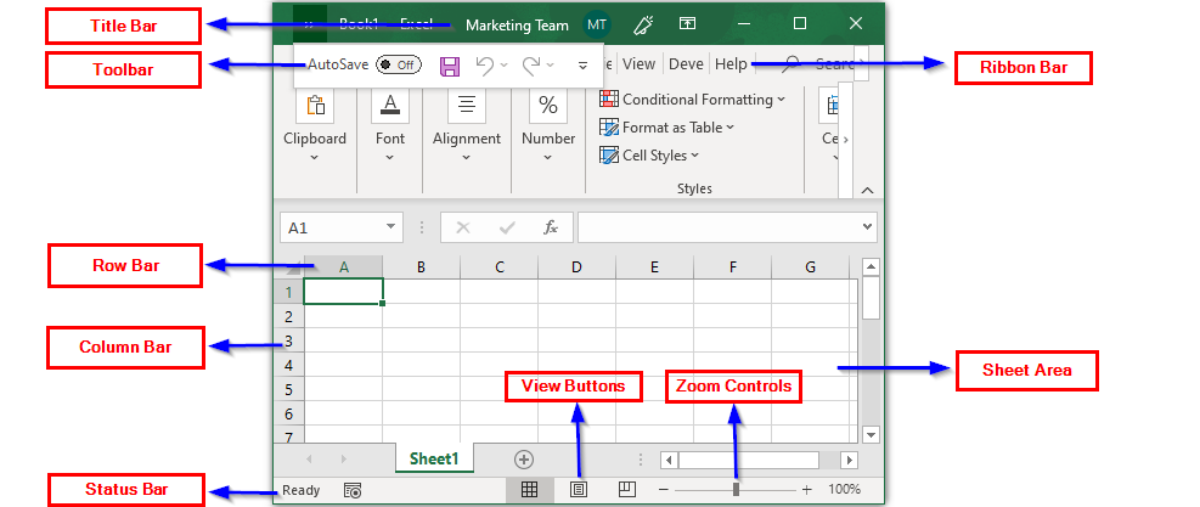
Understanding the Excel Interface
When you first open Microsoft Excel, you will be greeted with an interface that may appear overwhelming at first. However, once you understand the key components of the interface, navigating Excel becomes much easier.
The Excel interface consists of several elements, each serving a specific purpose in helping you work with your data effectively. Let’s take a closer look at these elements:
- Ribbon: The Ribbon is located at the top of the Excel window and is divided into tabs, such as Home, Insert, Page Layout, Formulas, Data, Review, and View. Each tab contains groups of related commands, making it easy for you to access the tools and features you need.
- Quick Access Toolbar: This toolbar is located above the Ribbon and contains frequently used commands, such as Save, Undo, and Redo. You can customize the Quick Access Toolbar to include additional commands that suit your workflow.
- Workbook: The workbook is the main document in Excel and is composed of individual worksheets. By default, a new workbook has three worksheets, but you can add or remove worksheets as needed.
- Worksheet: A worksheet is a grid of cells where you can enter and manipulate data. The worksheet tabs, located at the bottom of the screen, allow you to switch between different worksheets within the workbook.
- Formula Bar: The Formula Bar is located above the grid and displays the contents of the selected cell. You can enter formulas or edit the contents of cells directly in the Formula Bar.
- Columns and Rows: The grid is comprised of columns labeled with letters (A, B, C, etc.) and rows labeled with numbers (1, 2, 3, etc.). The intersection of a column and a row is called a cell, where you can input and manipulate data.
- Cell: A cell is the smallest unit in a worksheet and can contain various types of data, such as text, numbers, dates, or formulas.
- Status Bar: Located at the bottom of the Excel window, the Status Bar displays information about the current worksheet, such as the sum of selected cells or the average of a range.
By familiarizing yourself with the Excel interface, you will be able to work more efficiently and access the tools and features you need to accomplish your tasks. Understanding how to navigate through the Ribbon, utilize the Formula Bar, and work with worksheets and cells will allow you to harness the full power of Excel for your data management and analysis needs.
Creating a New Workbook
In Microsoft Excel, a workbook is a file that contains one or more worksheets, where you can enter, manipulate, and analyze data. Creating a new workbook is the first step to start working with Excel. Here’s how you can create a new workbook:
- Option 1: Opening Excel: The easiest way to create a new workbook is to open Microsoft Excel on your computer. Once Excel is open, a blank workbook will automatically be created for you.
- Option 2: Shortcut Key: Another quick way to create a new workbook is by using the keyboard shortcut Ctrl+N (Command+N on a Mac). Pressing this combination will instantly open a new workbook.
- Option 3: File Menu: You can also create a new workbook by clicking on the File menu at the top left corner of the Excel window. From the dropdown menu, select “New” and then choose “Blank Workbook.”
- Option 4: Opening from Template: In addition to a blank workbook, Excel offers various pre-designed templates that can help you jumpstart your work. By selecting “New from Template” in the File menu, you can browse through a collection of templates and choose the one that best suits your needs. Simply click on the desired template to open a new workbook based on that template.
Once you have created a new workbook, you can start entering data, applying formatting, and performing calculations. Excel allows you to add additional worksheets to the workbook by clicking on the plus icon (+) located near the worksheet tabs at the bottom of the screen. You can also insert, delete, and rearrange worksheets to organize your data effectively.
Remember to save your workbook frequently so that you can preserve your work. To save a new workbook for the first time, click on the File menu and select “Save As.” Choose a location on your computer and provide a name for the workbook. Excel will save the workbook in the default .xlsx format, which is compatible with other versions of Excel.
Creating a new workbook in Excel is the starting point for all your data management and analysis tasks. By understanding the different options to create a new workbook, you can quickly get started and take advantage of the powerful features Excel has to offer.
Saving and Opening Workbooks
In Microsoft Excel, saving and opening workbooks is essential for preserving your data and accessing it in the future. By following a few simple steps, you can easily save and open your Excel workbooks. Here’s how:
- Saving a Workbook: To save your workbook, click on the File menu at the top left corner of the Excel window. From the dropdown menu, select “Save” or use the shortcut key Ctrl+S (Command+S on a Mac). If you are saving the workbook for the first time, the “Save As” dialog box will appear. Choose the desired location on your computer and provide a name for your workbook. By default, Excel saves workbooks in the .xlsx format, which is compatible with other versions of Excel.
- Opening a Workbook: To open an existing workbook, click on the File menu and select “Open.” Alternatively, you can use the shortcut key Ctrl+O (Command+O on a Mac). The Open dialog box will appear, allowing you to browse your computer for the desired workbook. Once you locate the workbook, click on it and then click the “Open” button. Excel will open the workbook, and you can start working with the data.
- Recent Workbooks: Excel also provides a convenient way to access your recently opened workbooks. On the File menu, you will find a list of your most recently used workbooks under the “Recent” section. Simply click on the file name to open the workbook without navigating through the file system.
- AutoRecover: In case of unexpected computer shutdowns or Excel crashes, Excel has an AutoRecover feature that automatically saves a temporary backup of your workbook. When you open Excel after such an event, it will prompt you to recover any unsaved work. This can be a lifesaver in preventing data loss.
It is important to regularly save your work as you make changes to your workbook. This ensures that your data is protected and allows you to pick up where you left off at any time. Additionally, saving multiple versions of your workbook with different names or date stamps can be beneficial for tracking changes or creating backups.
By understanding the process of saving and opening workbooks in Excel, you can confidently manage your data and retrieve it efficiently whenever needed. Whether it’s preserving your work, accessing previous projects, or recovering unsaved data, Excel offers a range of options to help you work with your workbooks seamlessly.
The Basics of Entering Data
Entering data in Microsoft Excel is fundamental to creating and manipulating worksheets. Excel provides various options and techniques for entering data efficiently and accurately. Here’s a guide to help you understand the basics:
Entering Data Directly: To enter data directly into a cell, simply click on the desired cell and begin typing. The data you enter will appear in both the cell itself and the formula bar at the top of the screen. You can enter text, numbers, dates, or even formulas directly into the cells.
Copying and Pasting Data: Excel allows you to copy and paste data within a worksheet or between different worksheets or workbooks. To copy, select the cell or range of cells you want to copy, right-click, and choose “Copy” from the context menu. To paste, select the destination cell, right-click, and choose “Paste” or use the shortcut key Ctrl+V (Command+V on a Mac).
Filling Data: For repetitive data, Excel has a feature called AutoFill that allows you to quickly fill a series of cells with similar data. To use AutoFill, enter the initial value in a cell, hover your cursor over the bottom right corner of the cell until it turns into a crosshair, then click and drag to fill the desired range of cells.
Importing External Data: If you have data stored in a different format or source, such as a CSV file or a database, you can import that data into Excel. Click on the Data tab in the Ribbon, select “Get External Data,” and choose the appropriate import option to bring in the data.
Using Data Validation: Excel provides the option to apply data validation, which allows you to set rules and restrictions on the data entered into a cell. This helps maintain data integrity and prevents errors. To apply data validation, select the cell or range of cells, go to the Data tab in the Ribbon, and choose “Data Validation.”
Editing and Modifying Data: To edit or modify data in a cell, simply double-click on the cell or select the cell and begin typing. You can also press F2 on the keyboard to enter edit mode. Excel offers various editing options, such as cutting, copying, and pasting data, as well as undoing or redoing changes using the respective toolbar buttons or shortcut keys.
By mastering the basics of entering data in Excel, you can efficiently input and manage your information. Whether it’s manually typing in data, copying and pasting, filling a series, importing external data, or applying data validation, Excel provides the flexibility and functionality to streamline your data entry process.
Formatting Cells and Text
Formatting cells and text in Microsoft Excel can greatly enhance the visual appeal and organization of your data. Excel provides a wide range of formatting options to customize the appearance of cells, fonts, and other elements. Here are the basics of formatting cells and text:
Cell Formatting: Excel allows you to format cells to adjust their appearance and behavior. To format a cell, select the cell or range of cells you want to format. Right-click and choose “Format Cells” from the context menu or go to the Home tab in the Ribbon and use the Number Format dropdown. Here, you can choose from various options, including applying a specific number format, adjusting decimal places, and changing font colors or cell borders.
Font Formatting: Excel provides extensive options for formatting text within cells. You can change the font type, size, and color, as well as apply special effects such as bold, italic, underline, or strikethrough. To format text, select the cells containing the text, and use the font formatting options in the Home tab of the Ribbon. You can also use keyboard shortcuts, such as Ctrl+B for bold, Ctrl+I for italic, and Ctrl+U for underline.
Conditional Formatting: Conditional formatting is a powerful feature in Excel that allows you to format cells based on specific conditions or criteria. With conditional formatting, you can highlight cells that meet certain criteria, such as values above or below a specific threshold, duplicate values, or values that fall within a certain range. To apply conditional formatting, select the range of cells you want to format, go to the Home tab, and choose from the various options in the Conditional Formatting dropdown.
Alignment and Indentation: Excel provides options to align text within cells, allowing you to control the horizontal and vertical positioning of your data. The Alignment group in the Home tab provides buttons to align text left, center, or right, as well as to rotate text or wrap it within a cell. You can also use the Increase Indent and Decrease Indent buttons to adjust the indentation of cell contents.
Cell Styles: Excel offers predefined cell styles that can be applied to a range of cells to quickly change the appearance and formatting. Cell styles are available in the Home tab, and they include combinations of font formatting, border styles, and background colors. You can select a cell or range of cells and choose a style that best suits your needs.
By mastering the art of formatting cells and text in Excel, you can effectively present your data in a visually appealing and organized manner. Whether it’s adjusting cell formats, changing font styles, applying conditional formatting, aligning and indenting text, or using predefined cell styles, Excel offers a host of options to make your data stand out and communicate your message effectively.
Working with Rows, Columns, and Sheets
In Microsoft Excel, managing rows, columns, and sheets is essential for organizing and manipulating data effectively. Excel provides a range of options to help you work with these elements efficiently. Here’s a guide on working with rows, columns, and sheets:
Inserting Rows and Columns: To insert a row, right-click on the row number and select “Insert.” The new row will be inserted above the selected row. Similarly, to insert a column, right-click on the column letter and choose “Insert.” The new column will be inserted to the left of the selected column. You can also use the Insert command in the Home tab of the Ribbon to insert rows and columns.
Deleting Rows and Columns: To delete a row or column, right-click on the row number or column letter and select “Delete.” The selected row or column will be removed, and the data below or to the right will shift up or left respectively. You can also use the Delete command in the Home tab to delete rows and columns.
Adjusting Row Height and Column Width: Excel allows you to adjust the height of rows and the width of columns to accommodate your data. To adjust the height of a row, hover your cursor over the row number until it turns into a double arrow, then click and drag to increase or decrease the row height. Similarly, to adjust the width of a column, hover your cursor over the column letter until it turns into a double arrow, then click and drag to increase or decrease the column width.
Organizing Sheets: Excel workbooks can contain multiple sheets, which are represented as tabs at the bottom of the screen. To add a new sheet, click on the plus icon (+) next to the existing sheet tabs. To delete a sheet, right-click on the sheet tab and select “Delete.” You can also rename sheets by double-clicking on the sheet tab and entering a new name. To move sheets, click and drag the sheet tab to the desired position.
Grouping and Ungrouping Rows and Columns: Excel allows you to group rows or columns together, making it easy to collapse or expand them for better organization. To group, select the rows or columns you want to group, right-click, and choose “Group.” To ungroup, select the grouped rows or columns, right-click, and choose “Ungroup.”
Freezing Rows and Columns: When working with large datasets, it can be helpful to freeze certain rows or columns so that they remain visible as you scroll through the worksheet. To freeze rows, select the row below the desired frozen rows, go to the View tab in the Ribbon, and click on “Freeze Panes” and choose “Freeze Panes.” To freeze columns, select the column to the right of the desired frozen columns and follow the same steps.
By understanding how to work with rows, columns, and sheets in Excel, you can effectively organize and manipulate your data. Whether it’s inserting or deleting rows and columns, adjusting row height and column width, grouping and ungrouping data, or managing multiple sheets, Excel provides the versatility and functionality to streamline your workflow and keep your data organized.
Working with Formulas and Functions
In Microsoft Excel, formulas and functions are powerful tools that allow you to perform calculations and automate tasks. Whether you need to calculate simple sums or perform complex data analysis, Excel provides a wide range of built-in functions to help you achieve your goals. Here’s a guide on working with formulas and functions:
Entering Formulas: To enter a formula in Excel, begin by selecting the cell where you want the result to appear. Type the equals sign (=) followed by the formula. You can use mathematical operators such as addition (+), subtraction (-), multiplication (*), and division (/), as well as parentheses to control the order of operations.
Built-in Functions: Excel offers a vast library of built-in functions that perform specific operations on your data. These functions can range from simple calculations like SUM, AVERAGE, and COUNT to more advanced functions like VLOOKUP, IF, and CONCATENATE. To use a function, type the equals sign (=), followed by the function name and the required arguments within parentheses. Excel provides autocompletion and built-in help to guide you in using functions correctly.
Referencing Cells: Formulas can reference the values in other cells to perform calculations. To reference a cell, simply enter the cell’s address, such as A1 or B5, within the formula. You can also click on the desired cell while entering the formula to automatically reference it. Excel allows you to use cell references in complex formulas and functions to perform calculations on dynamically changing data.
Using Operators and Functions Together: Excel allows you to combine operators and functions within a single formula. For example, you can use the SUM function to add a range of cells and then multiply the result by a constant value using the multiplication operator (*). This flexibility allows for complex calculations using a combination of mathematical operations and functions.
AutoFill for Formulas: Excel’s AutoFill feature can quickly copy formulas and functions down a column or across a row. Simply enter the formula in the first cell, hover your cursor over the bottom right corner until it turns into a crosshair, and then click and drag to copy the formula to the desired range.
Debugging Formulas: If you encounter errors in your formulas, Excel provides error checking and debugging tools to help you identify and resolve issues. The Formula Auditing tools in the Formulas tab of the Ribbon allow you to trace precedents, dependents, and errors within your formulas to troubleshoot and fix any problems.
By mastering the use of formulas and functions in Excel, you can perform a wide range of calculations and automate tasks efficiently. Whether it’s performing basic arithmetic operations, utilizing built-in functions, referencing cells, combining operators and functions, or using AutoFill and debugging tools, Excel empowers you to analyze and manipulate your data effectively.
Viewing and Printing Worksheets
In Microsoft Excel, viewing and printing worksheets accurately is essential for reviewing and sharing your data. Excel provides various options to adjust the view of your worksheet and customize the print settings. Here’s a guide to help you effectively view and print your worksheets:
Zooming and Scaling: Excel allows you to adjust the zoom level of your worksheet to view more or less content on the screen. In the bottom-right corner of the Excel window, you will find a zoom slider that you can drag left or right to adjust the zoom level. Additionally, you can use the Zoom commands in the View tab of the Ribbon to set a specific zoom percentage. Excel also provides options for scaling the printout to fit on a specific number of pages.
Page Layout View: Excel’s Page Layout view provides a more accurate representation of how your worksheet will look when printed. This view allows you to adjust margins, add headers and footers, and control page breaks. To switch to the Page Layout view, click on the View tab in the Ribbon and select “Page Layout.”
Page Break Preview: The Page Break Preview view in Excel allows you to see your worksheet broken down into pages, including where page breaks occur. This view helps you adjust the layout of your data to ensure it fits neatly on the printed page. To switch to the Page Break Preview view, click on the View tab in the Ribbon and select “Page Break Preview.”
Page Setup: Excel’s Page Setup dialog box provides extensive options for customizing the appearance and layout of your worksheet when printed. From the Page Setup dialog box, you can adjust margins, page orientation (portrait or landscape), paper size, print area, headers and footers, and much more. To access the Page Setup dialog box, click on the Page Layout tab in the Ribbon and select “Page Setup” in the Page Setup group.
Printing Options: Excel offers various printing options to suit your needs. You can control what prints by selecting specific cells or ranges, or you can print the entire worksheet. Excel also provides options for printing a selection of worksheets or the entire workbook. To access the print settings, click on the File menu and select “Print.” Review the settings in the Print dialog box and adjust as needed before sending the print job to your printer.
Print Preview: Before you print your worksheet, it’s always a good idea to review the printout using the Print Preview feature. Excel’s Print Preview allows you to see how your worksheet will look when printed, including page breaks, margins, headers, footers, and other settings. To access Print Preview, click on the File menu and select “Print.” The worksheet will be displayed in the Print Preview pane, where you can scroll through the pages and make any necessary adjustments before printing.
By effectively viewing and printing your worksheets in Excel, you can ensure the accurate representation of your data on paper. Whether it’s adjusting zoom levels, utilizing Page Layout view and Page Break Preview, customizing settings in the Page Setup dialog box, selecting printing options, or previewing the printout using Print Preview, Excel provides the tools you need to present your data in a professional and organized manner.
Using AutoFill and Flash Fill
In Microsoft Excel, the AutoFill and Flash Fill features are powerful tools that can save you time and effort when working with repetitive or patterned data. These features allow you to quickly fill in data series, make data transformations, and automate common data entry tasks. Here’s a guide on how to use AutoFill and Flash Fill in Excel:
AutoFill: Excel’s AutoFill feature enables you to automatically fill a series of cells with a pattern or sequence. To use AutoFill, enter the starting value in a cell and then hover your cursor over the bottom right corner of the cell until it turns into a crosshair. Click and drag to fill the desired range with the AutoFill series. Excel can recognize and generate various types of series, including numbers, dates, weekdays, months, or even custom series defined by your own pattern.
Flash Fill: Flash Fill goes a step further by automatically extracting or transforming data based on a pattern it recognizes. This feature can save you significant time when manipulating data in a structured format. For example, if you have a column with first names and another column with last names, you can use Flash Fill to extract the first names or concatenate the first and last names into a single column. Excel intelligently identifies the pattern based on the examples you provide and automatically fills in the rest of the data. To use Flash Fill, enter the desired transformation in the adjacent column, press Ctrl+E (or Command+E on a Mac), and Excel will generate the remaining data.
Using AutoFill for Formulas: In addition to filling a series of values, AutoFill can be used to quickly copy formulas across a range of cells. Enter the formula in the first cell, then use AutoFill to copy and paste the formula into the desired range. Excel automatically adjusts the cell references in the formula to match the relative positions of the cells, saving you from having to manually update each formula.
Customizing AutoFill Options: Excel provides options to customize the behavior of AutoFill. You can access these options by going to the File menu, selecting “Options,” and choosing “Advanced.” In the Advanced Options, find the Editing Options section, where you can enable or disable AutoFill and modify the default behavior of the AutoFill series.
Control Flash Fill Patterns: While Flash Fill is designed to automatically recognize patterns in your data, you can also control its behavior by providing examples and using additional formatting or functions. Excel allows you to edit individual cells if Flash Fill does not generate the desired result. You can also undo or redo Flash Fill actions and clear Flash Fill suggestions using the Flash Fill Options button that appears next to the filled data.
By utilizing the AutoFill and Flash Fill features in Excel, you can significantly speed up your data entry and transformation tasks. Whether you need to fill a series of cells, extract or transform data, or copy formulas, Excel’s AutoFill and Flash Fill capabilities help you work more efficiently and automate common data-related tasks.
Sorting and Filtering Data
In Microsoft Excel, sorting and filtering data is essential for organizing and analyzing large sets of information. Excel provides powerful tools that allow you to quickly sort your data in ascending or descending order, as well as apply filters to display specific subsets of your data. Here’s a guide on how to sort and filter data in Excel:
Sorting Data: To sort data in Excel, select the range of cells you want to sort, including any headers if applicable. Then, go to the Data tab in the Ribbon and click on the “Sort” button. In the Sort dialog box, specify the column to sort by and choose the sort order (ascending or descending). You can sort by multiple columns by clicking on the “Add Level” button and selecting additional sort criteria.
Custom Sorting: Excel also allows you to perform custom sorts based on specific criteria. For example, you can sort alphabetically by the last name of a list of names. To perform a custom sort, select the range of cells, go to the Data tab, click on the “Sort” button, and choose “Custom Sort” from the dropdown menu. In the Custom Sort dialog box, define your custom sort criteria by specifying the column to sort and the desired sort order or criteria.
Filtering Data: Excel’s filtering feature enables you to display specific subsets of data based on specified criteria. To apply a filter, select the range of cells, go to the Data tab, and click on the “Filter” button. Excel will add filter arrows to each column header. Click on the filter arrow to display a dropdown menu, where you can select or deselect specific values to filter the data accordingly. You can also use the “Sort A to Z” or “Sort Z to A” options in the filter menu to sort the filtered data.
Advanced Filtering: Excel provides advanced filtering options that allow you to apply complex criteria for filtering your data. By selecting the range of cells, going to the Data tab, clicking on the “Advanced” button in the Sort & Filter group, and entering your specific criteria in the Advanced Filter dialog box, you can create custom filtering conditions based on multiple columns and complex logical operators.
Clearing Filters and Sorting: To remove filters and show all the data again, go to the Data tab, click on the “Filter” button, and select “Clear Filter.” To remove sorting and return to the original order, go to the Data tab, click on the “Sort” button, and choose “Clear” in the Sort dialog box.
By mastering the sorting and filtering capabilities in Excel, you can easily organize and analyze your data. Whether you need to sort data in a specific order or display subsets of data based on certain criteria, Excel provides a range of tools to help you efficiently manage and manipulate your information.
Using Conditional Formatting
In Microsoft Excel, conditional formatting is a powerful tool that allows you to highlight and format cells based on predefined rules or conditions. This feature helps you analyze and draw attention to specific patterns, trends, or outliers within your data. Here’s a guide on how to use conditional formatting in Excel:
Applying Conditional Formatting: To apply conditional formatting, select the range of cells you want to format. Then, go to the Home tab in the Ribbon and click on the “Conditional Formatting” button. From the dropdown menu, you can choose from various predefined formatting options, such as highlighting cells that contain specific text or values, color scales, data bars, icon sets, or even creating custom rules based on formulas.
Highlighting Cells: Conditional formatting allows you to highlight cells based on specific conditions. For example, you can highlight cells that contain values above a certain threshold or cells that meet a specific criteria set by a formula. By selecting the appropriate conditional formatting rule, you can easily draw attention to relevant data in your worksheet.
Color Scales and Data Bars: Excel’s conditional formatting also provides color scales and data bars to visually represent the relative values of cells within a range. Color scales allow you to assign different colors to cells based on their values, making it easier to identify high and low values or patterns within your data. Data bars, on the other hand, create horizontal bars within cells to represent the magnitude of the values they contain.
Icon Sets: Icon Sets are another type of conditional formatting available in Excel. Icon Sets allow you to display icons or symbols next to cells based on their values. For example, you can assign arrows pointing up, down, or sideways to represent the trend of values within a range. This can be particularly useful for visualizing data trends or performance indicators.
Editing and Managing Conditional Formatting Rules: Excel allows you to easily edit and manage conditional formatting rules. To modify a rule, select the range of cells with the applied conditional formatting, go to the Home tab, click on the “Conditional Formatting” button, and choose “Manage Rules” from the dropdown menu. In the Conditional Formatting Rules Manager, you can add, edit, or delete existing rules, as well as change the order in which they are applied.
Clearing Conditional Formatting: If you want to remove conditional formatting from a range of cells, select the cells, go to the Home tab, click on the “Conditional Formatting” button, and choose “Clear Rules” from the dropdown menu. You can remove all conditional formatting or clear specific rules applied to the selected cells.
By effectively using conditional formatting in Excel, you can highlight and analyze your data in a visually appealing and meaningful way. Whether you choose to highlight cells, apply color scales or data bars, or use icon sets, conditional formatting helps to draw attention to important insights and trends, making it easier to interpret and analyze your data.
Creating and Formatting Charts
In Microsoft Excel, charts are powerful visual representations of data that allow you to analyze and present information effectively. Excel offers a wide range of chart types and customization options to create visually appealing and informative charts. Here’s a guide on how to create and format charts in Excel:
Creating a Chart: To create a chart in Excel, select the range of data you want to include in the chart, including any column or row labels. Then, go to the Insert tab in the Ribbon and click on the desired chart type, such as Column, Line, Pie, or Bar. Excel will generate a default chart based on the selected data.
Customizing Chart Elements: Excel provides extensive customization options for chart elements. With the chart selected, you can use the Chart Design, Chart Layout, and Format tabs in the Ribbon to modify various aspects of the chart, such as adding or removing chart titles, axis labels, legends, gridlines, and data labels. You can also choose different chart styles, color schemes, or 3D effects to suit your preferences.
Switching Chart Types: Excel allows you to easily switch between different chart types to find the most suitable representation of your data. With the chart selected, go to the Design tab in the Ribbon and click on the “Change Chart Type” button. Excel will present you with a gallery of chart types to choose from. Select the desired chart type and customize its elements as needed.
Formatting Chart Data: You can easily format the data series within a chart to highlight specific data points or trends. With the chart selected, click on a data series to activate it, and then right-click to access formatting options. You can modify the color, marker style, and line style of each data series to enhance the visual representation and emphasize key information.
Adding Chart Elements: Excel allows you to add additional chart elements to enhance the clarity and understanding of your data. With the chart selected, go to the Chart Layout tab in the Ribbon and click on the “Add Chart Element” button. From the dropdown menu, you can choose to add data labels, trendlines, error bars, and more. These elements can provide valuable insights and context to your chart.
Changing Chart Data: If you need to modify or update the data in your chart, you can easily do so in Excel. Simply edit the values in the original data range, and the chart will automatically reflect the changes. You can also resize or move the chart within the worksheet to better fit your needs.
By utilizing the charting features in Excel, you can create visually compelling and informative charts to communicate your data effectively. Whether you’re customizing chart elements, switching chart types, formatting data series, adding elements, or updating chart data, Excel provides the versatility and flexibility to create professional and visually appealing charts.
Using Basic Excel Functions
In Microsoft Excel, functions are prebuilt formulas that perform specific calculations or actions on data. Excel offers a wide array of basic functions that can help you perform common mathematical, statistical, logical, and text operations. Here’s a guide on how to use basic Excel functions:
SUM Function: The SUM function allows you to add up a range of numbers. You can specify individual cells, cell ranges, or even include mathematical operators within the function. For example, =SUM(A1:A5) will give you the sum of the values in cells A1 through A5.
AVERAGE Function: The AVERAGE function calculates the average of a range of numbers. Like the SUM function, you can specify individual cells or cell ranges. For example, =AVERAGE(B1:B5) will give you the average of the values in cells B1 through B5.
COUNT Function: The COUNT function counts the number of cells that contain numerical values within a specified range. For example, =COUNT(C1:C5) will give you the count of cells in the range C1 through C5 that contain numbers.
MAX and MIN Functions: The MAX and MIN functions find the maximum and minimum values within a range, respectively. For example, =MAX(D1:D5) will give you the largest value in the range D1 through D5, whereas =MIN(D1:D5) will give you the smallest value.
IF Function: The IF function allows you to perform conditional calculations based on specified criteria. It evaluates a logical condition and returns one value if the condition is true, and another value if the condition is false. For example, =IF(A1>10, “Greater than 10”, “Less than or equal to 10”) will check if the value in cell A1 is greater than 10, and return the corresponding message.
CONCATENATE Function: The CONCATENATE function enables you to combine multiple text strings into one string. For example, =CONCATENATE(“Hello”, ” “, “World”) will result in the string “Hello World”. This function is useful for joining text from different cells or adding additional text to cell values.
DATE Function: The DATE function allows you to create a date using the year, month, and day values provided as arguments. For example, =DATE(2022, 12, 31) will return the date December 31, 2022. This function is helpful for performing calculations or creating date-based formulas.
TRIM Function: The TRIM function removes any extra spaces from a text string, excluding single spaces between words. This can help clean up data or standardize formatting. For example, =TRIM(” Hello “) will return “Hello” by removing the extra spaces on both sides.
By familiarizing yourself with basic Excel functions, you can perform a wide range of calculations and operations on your data more efficiently. Whether you’re adding up values, finding averages, counting cells, evaluating conditions, combining text, manipulating dates, or cleaning up data, Excel’s functions provide powerful tools to simplify your work and enhance data analysis.
Summarizing and Analyzing Data with PivotTables
In Microsoft Excel, PivotTables are valuable tools for summarizing and analyzing large amounts of data. They allow you to extract meaningful insights by organizing and summarizing data into a concise and digestible format. Here’s a guide on how to use PivotTables to summarize and analyze your data:
Creating a PivotTable: To create a PivotTable, ensure your data is properly organized with column headers. Select the range of cells you want to analyze, go to the Insert tab in the Ribbon, and click on the “PivotTable” button. Choose whether to place the PivotTable on a new worksheet or an existing one.
Adding Fields: In the PivotTable Field List pane, you will see a list of all the column headers from your data source. Drag and drop the relevant fields into the Rows, Columns, and Values areas to define the structure of your PivotTable. You can summarize data by different categories and apply calculations such as sum, average, count, or more complex formulas.
Modifying the PivotTable: You can easily modify and customize your PivotTable to meet your analysis needs. Dragging and rearranging fields in the Field List pane allows you to change the layout of the PivotTable. You can also add or remove fields on the fly to include or exclude data from the analysis.
Grouping Data: Excel allows you to group data within a PivotTable to further analyze and summarize information. For example, you can group dates by months or years, or group numeric data into specific ranges. Grouping data provides a more compact and organized view of the information.
Applying Filters: PivotTables offer filtering capabilities to focus on specific subsets of data. By applying filters to the fields in your PivotTable, you can narrow down the analysis to particular categories or values of interest. This allows for deeper examination of data patterns and trends.
Updating PivotTable Data: When your underlying data changes or expands, you can easily update the PivotTable. Right-click on the PivotTable, select “Refresh,” and Excel will retrieve and summarize the latest data. This ensures that your analysis is always based on the most up-to-date information.
Formatting and Styling: Excel provides various formatting options to enhance the visual representation of your PivotTable. You can customize the layout, apply different formats to cells, add conditional formatting, and use styles to make the PivotTable more visually appealing and accessible.
PivotTables enable you to analyze and extract insights from large datasets efficiently. By summarizing data, applying calculations, grouping information, and applying filters, PivotTables provide a dynamic and interactive way to understand and interpret your data effectively. Excel’s PivotTable feature is a valuable tool for data analysis, reporting, and decision-making in various professional and personal contexts.
Tips and Tricks for Excel Efficiency
Microsoft Excel is a powerful tool for data management and analysis. To enhance your productivity and efficiency, here are some useful tips and tricks:
Keyboard Shortcuts: Excel offers a wide range of keyboard shortcuts to perform common tasks quickly. Learn commonly used shortcuts like Ctrl+C for copying, Ctrl+V for pasting, Ctrl+S for saving, Ctrl+Z for undoing actions, and Ctrl+Y for redoing actions. Familiarizing yourself with these shortcuts can significantly speed up your workflow.
Autofill and Flash Fill: Take advantage of Excel’s Autofill feature to quickly fill in data series or copy formulas across a range of cells. For more complex data transformations, use Flash Fill to automatically extract or transform data based on patterns. These features can save you time and effort when working with repetitive or structured data.
Customizing the Quick Access Toolbar: Customize the Quick Access Toolbar at the top of the Excel window to include commonly used commands. Simply right-click on any command in the Ribbon and choose “Add to Quick Access Toolbar.” This allows you to access frequently used commands with just one click.
Using Named Ranges: Assign names to ranges of cells to make your formulas easier to read and understand. Instead of referring to cells by their addresses (e.g., A1:B10), you can use names that represent their purpose (e.g., SalesData). This makes your formulas more intuitive and helps in navigating large worksheets.
Conditional Formatting: Utilize conditional formatting to highlight important trends, outliers, or patterns in your data. Applying color scales, data bars, or icon sets can make it easier to visually analyze and interpret information. Use different formatting options to create customized visual cues.
Working with Multiple Worksheets: Manage multiple worksheets efficiently by using group sheets, linking cells between sheets, and utilizing color-coded tabs for easy identification. You can also insert or delete multiple worksheets at once by selecting multiple sheets using Ctrl+Click.
Using PivotTables: PivotTables are powerful tools for summarizing and analyzing data. Master the art of creating PivotTables, customizing them, and using filters and grouping to gain meaningful insights from your data. PivotTables help you organize, analyze, and present data effectively.
Excel Functions and Formulas: Familiarize yourself with commonly used Excel functions and formulas such as SUM, AVERAGE, VLOOKUP, and IF. Understanding and utilizing these functions can simplify complex calculations and save time troubleshooting errors.
Excel Templates and Add-Ins: Explore the wide variety of Excel templates and add-ins available online. These resources can help streamline your work by providing pre-designed spreadsheets, specialized tools, and expanded functionalities.
By leveraging these tips and tricks, you can enhance your proficiency and efficiency in using Microsoft Excel. Mastering keyboard shortcuts, utilizing autofill and conditional formatting, customizing toolbars, and harnessing the power of PivotTables and functions can significantly improve your productivity and effectiveness in working with data in Excel.