
The Basics of the SUM Function
The SUM function is one of the most commonly used functions in Microsoft Excel. It is a powerful tool that allows you to quickly calculate the sum of a range of cells. Whether you need to sum a column, a row, or a group of cells, the SUM function can save you time and effort. In this section, we will explore the fundamentals of using the SUM function.
To use the SUM function, you simply need to select the range of cells that you want to sum. You can do this by highlighting the cells with your mouse or by manually entering the range in the formula bar. Once you have selected the cells, you can begin building your SUM formula.
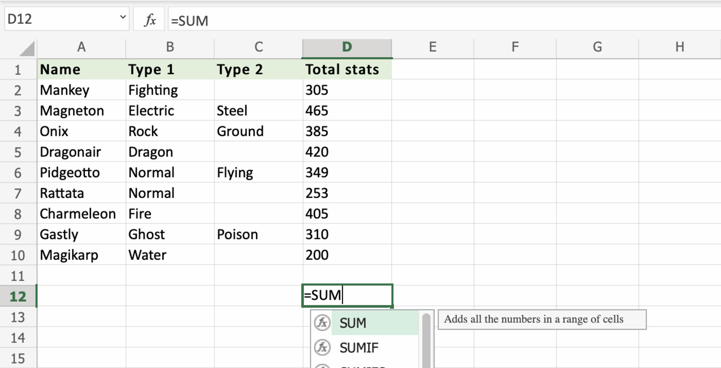
The syntax of the SUM function is straightforward. It consists of the function name followed by an opening parenthesis, the range of cells or values to be summed, and a closing parenthesis. For example, to sum the values in cells A1 to A5, you would enter the following formula: =SUM(A1:A5).
When using the SUM function, keep in mind that it only works with numerical values. If any of the cells in the selected range contain non-numeric data or errors, the function will ignore those cells and calculate the sum of the remaining numeric values. Additionally, the SUM function treats empty cells as zeros, so they will be included in the sum.
By default, the SUM function calculates the sum in the cell where the formula is entered. However, you can also specify a different cell to display the result. Simply select the cell where you want the sum to appear before entering the formula.
Summing a Column with the SUM Function
Summing a column of numbers in Excel is a task that can be easily accomplished using the SUM function. Whether you have a small or large dataset, the SUM function can efficiently calculate the total sum of all the values in a single column.
To sum a column using the SUM function, start by selecting a cell where you want the sum to appear. Then, enter the formula =SUM(A:A) in the selected cell, where “A” represents the column letter you want to sum.
If you only want to sum a specific range of cells in the column, you can modify the formula accordingly. For example, if you want to sum values from cell A2 to A10, you would use the formula =SUM(A2:A10).
It is worth mentioning that when you use the SUM function to sum a column, make sure that the column contains only numerical values. If there are any non-numeric data or errors within the column, the SUM function will ignore them and calculate the sum of the remaining numeric values.
Additionally, if you have a column that includes both numbers and text, you can use other functions like the SUMIF or SUMIFS functions to selectively sum cells based on certain criteria. These functions allow you to specify conditions and only include values that meet those conditions in the sum.
Once you have entered the SUM formula, press Enter, and the sum of the column will be displayed in the selected cell. Excel will automatically update the sum if any values in the column change.
By utilizing the SUM function to sum columns in Excel, you can easily analyze and understand the data without the need for manual calculations. It saves time, reduces the chance of errors, and allows you to focus on other important tasks.
Summing a Row with the SUM Function
Summing a row of numbers in Excel can be done effortlessly using the SUM function. Whether you have a small or large dataset, the SUM function allows you to quickly calculate the total sum of all the values in a row.
To sum a row using the SUM function, select the cell where you want the sum to appear. Then, enter the formula =SUM(1:1) in the selected cell, where “1” represents the row number you want to sum.
If you want to sum a specific range of cells in the row, modify the formula accordingly. For example, to sum values from column B to column G in row 1, you would use the formula =SUM(B1:G1).
It’s important to note that when summing a row using the SUM function, ensure that the row contains only numerical values. Non-numeric data or errors within the row will be ignored by the SUM function, calculating the sum of the remaining numeric values only.
Furthermore, if your row contains a combination of numbers and text, you can utilize other functions such as SUMIF or SUMIFS to selectively sum cells based on specific criteria. These functions enable you to set conditions and include only values that meet those conditions in the sum.
After entering the SUM formula, hit Enter, and the sum of the row will be displayed in the selected cell. If any values in the row change, Excel will automatically update the sum accordingly.
By utilizing the SUM function to sum rows in Excel, you can efficiently analyze and interpret data without the need for manual calculations. It saves time, reduces the risk of errors, and allows you to focus on more critical tasks.
Using the AutoSum Button to Sum Columns or Rows
Excel provides a handy tool called the AutoSum button that allows you to quickly and easily sum columns or rows without having to manually enter the SUM formula. The AutoSum button can save you time and effort, especially when dealing with large datasets.
To use the AutoSum button, follow these simple steps:
1. Select the cell where you want the sum to appear. This could be a cell below a column or to the right of a row that you want to sum.
2. Click on the AutoSum button situated in the Editing group on the Home tab of the Excel ribbon. The button looks like the Greek letter sigma (∑).
3. Excel will automatically detect the range of cells above or to the left of the selected cell and insert the SUM formula accordingly.
4. Press Enter, and the sum of the column or row will be displayed.
The AutoSum button is highly versatile and can be used to sum multiple columns or rows simultaneously. Simply select the cells below the columns or to the right of the rows that you want to sum before clicking the AutoSum button. Excel will insert the appropriate SUM formulas for each selected column or row, giving you quick access to the sums.
It’s important to note that the AutoSum button is a great tool for basic summing tasks. However, if you need more flexibility or want to include specific criteria in your calculations, you may need to use the SUM function with manual adjustments.
By utilizing the AutoSum button, you can streamline your workflow and simplify the process of summing columns or rows in Excel. It’s a time-saving feature that allows you to focus on analyzing and interpreting your data effectively.
Summing Multiple Columns or Rows with the SUM Function
When working with Excel, it is common to come across situations where you need to sum multiple columns or rows together. Fortunately, the SUM function in Excel allows you to easily accomplish this task, making it a powerful tool for data analysis and calculation.
To sum multiple columns or rows with the SUM function, you can use the colon operator to specify a range of cells. For example, to sum columns A to C, you would use the formula =SUM(A:C). Similarly, to sum rows 1 to 5, you would use the formula =SUM(1:5).
By using the SUM function with a range of cells, Excel will automatically calculate the sum of each column or row and provide the total in the selected cell. This method is particularly useful when dealing with large datasets or when you need to perform calculations on multiple rows or columns simultaneously.
In addition to using the colon operator, you can also use the comma to separate individual ranges within the SUM function. For example, if you wanted to sum columns A to C and columns E to G, you would use the formula =SUM(A:C, E:G). This allows you to sum non-contiguous columns or rows efficiently.
Furthermore, you can expand on this functionality by using other functions in conjunction with the SUM function. For example, you can use the SUMIF or SUMIFS function to sum specific columns or rows based on certain criteria. This enables you to perform conditional sums and extract valuable insights from your data.
Whether you need to sum a few adjacent columns or rows or perform complex calculations on non-contiguous ranges, the SUM function in Excel provides a flexible and efficient solution. It saves time, reduces manual errors, and allows you to perform data analysis with ease.
Using the SUM Function with Conditions or Criteria
Excel’s SUM function becomes even more powerful when combined with conditions or criteria. By incorporating criteria into the formula, you can selectively sum only the cells that meet specific requirements, allowing for more specialized data analysis and calculations.
The SUM function can be enhanced with the use of the SUMIF or SUMIFS functions. The SUMIF function allows you to specify a single criterion, whereas the SUMIFS function enables you to specify multiple criteria.
To use the SUMIF function, you need to provide three arguments: the range of cells to evaluate, the criterion or condition to be met, and the range of cells to sum. For example, to sum values in column A that are greater than 10, you would use the formula: =SUMIF(A:A, ">10").
If you have multiple criteria to consider, you can utilize the SUMIFS function. This function allows you to specify multiple ranges to evaluate and their respective criteria. For instance, to sum values in column A that are greater than 10 and in column B that are less than 5, you would use the formula: =SUMIFS(A:A, ">10", B:B, "<5").
With the combination of the SUM function and criteria, you can perform complex calculations and gain valuable insights from your data. Whether you need to sum sales figures based on specific regions, sum expenses based on certain categories, or perform any other custom calculations, the SUM function with conditions or criteria is a powerful tool.
Remember to ensure that the criteria you provide in the formula are appropriate for the data you are working with. Additionally, double-check the range of cells you specify to ensure that it covers the necessary data.
By using the SUM function with conditions or criteria, you can efficiently analyze and summarize your data based on specific requirements. This provides a more comprehensive understanding of your data and allows for targeted data analysis and reporting.
Using the SUM Function with Multiple Worksheets
Excel allows you to work with multiple worksheets within a single workbook, and the SUM function can be used across these worksheets to consolidate and calculate data from different sources. This powerful feature enables you to perform complex calculations and analysis, even when your data is spread across multiple sheets.
To use the SUM function with multiple worksheets, you have a couple of options:
1. Manually reference each worksheet: In this method, you would enter the SUM formula with references to specific cells or ranges on each worksheet. For example, to sum cell A1 from Sheet1 and cell B1 from Sheet2, you would use the formula =SUM(Sheet1!A1, Sheet2!B1). This method allows for precise control over which cells or ranges are included in the sum.
2. Use the 3D cell reference: This method is especially useful when you want to sum the same cell or range across multiple worksheets. You can use the 3D cell reference by using the syntax =SUM(Sheet1:Sheet3!A1). This formula will sum cell A1 from Sheet1, Sheet2, and Sheet3. If you have additional sheets, you can extend the range accordingly. This method simplifies the formula and makes it easier to sum data from a large number of worksheets.
It's crucial to note that when summing across multiple worksheets, each worksheet must be in the same workbook. Additionally, ensure that the references are correct, including the worksheet names and the cell or range references.
By using the SUM function with multiple worksheets, you can consolidate and summarize data from various sources efficiently. This capability is particularly valuable when dealing with large datasets or when you need to perform calculations and analysis across multiple related sheets.
Remember to review and update your formulas as necessary if there are any changes in the source data or the number of worksheets. This will ensure accurate calculation results.
Using the SUM function with multiple worksheets enhances the capabilities of Excel, allowing you to consolidate and analyze data seamlessly across different sheets within a workbook.
Tips and Tricks for Using the SUM Function Efficiently
The SUM function in Excel is a powerful tool for calculating totals, and by implementing a few tips and tricks, you can maximize its efficiency and make your data analysis process more streamlined. Here are some useful tips to consider when using the SUM function:
1. Use keyboard shortcuts: Instead of manually typing out the sum formula, use the Alt + = keyboard shortcut to quickly insert the AutoSum function. This can save you time, especially when summing large datasets.
2. Exclude non-numeric data: When using the SUM function, ensure that the selected cells contain only numeric data. Non-numeric values, including text and errors, will be ignored by the function. If you encounter an issue with the sum result, check for any non-numeric data in the selected range.
3. Utilize named ranges: If your dataset has a specific range that needs to be summed frequently, consider defining a named range. By assigning a name to a range of cells, you can simply use the range name in the SUM function instead of manually selecting the cells each time.
4. Combine SUM with other functions: The SUM function can work seamlessly with other functions such as IF, COUNTIF, and AVERAGE. By combining these functions, you can perform more complex calculations and analyze data based on specific conditions or criteria.
5. Utilize auto-fill: Excel's auto-fill feature is a handy tool when working with large datasets. You can use it to quickly copy the SUM formula across multiple cells or ranges, saving you the effort of writing the formula repeatedly.
6. Link between worksheets: If you need to sum data from different worksheets, consider using the 3D cell reference or linking formulas to consolidate the data into a single worksheet. This allows for easier management and analysis of the summed values.
7. Exclude outliers: If you want to exclude specific values from the sum calculation, you can incorporate logical operators within the SUM formula. For example, you can use the SUMIF or SUMIFS function to sum only the cells that meet certain criteria, allowing for more precise data analysis.
By applying these tips, you can enhance your efficiency and accuracy when using the SUM function in Excel. These techniques not only save time but also enable more advanced calculations and analysis, making your data management tasks more efficient and effective.
Common Errors and Troubleshooting Tips for Summing Columns or Rows
While using the SUM function in Excel to sum columns or rows, it's not uncommon to encounter errors or unexpected results. Understanding and troubleshooting these issues is essential for accurate calculations and analysis. Here are some common errors and important troubleshooting tips to consider:
1. #VALUE! error: This error occurs when the selected range contains non-numeric values or cells with errors. Make sure to exclude these cells or correct any errors in the range to avoid this error.
2. #REF! error: The #REF! error appears when the referenced cells in the sum formula have been deleted, moved, or renamed. Double-check the cell references to ensure they are correct and point to valid ranges.
3. Incorrect range selection: Selecting the wrong range of cells can lead to incorrect sum results. Carefully check the selected range and adjust it as needed to accurately sum the desired columns or rows.
4. Hidden or filtered cells: Hidden or filtered cells are often overlooked when summing columns or rows. Ensure that any hidden or filtered cells that should be included in the sum are visible or unfiltered before performing the calculation.
5. Circular reference error: If the selected range for summing includes the cell containing the SUM formula itself, it will result in a circular reference error. Avoid including the formula cell in the range to resolve this issue.
6. Multiple instances of SUM within a single cell: Avoid using multiple instances of the SUM function within a single cell. It can lead to confusion and incorrect results. Instead, use separate cells for each sum calculation to maintain clarity and accuracy.
7. Incorrect syntax: Ensure that the syntax of the SUM formula is correct. It should follow the pattern =SUM(range) or =SUM(number1, number2, ...). Double-check the formula for any missing or incorrect parentheses, commas, or range references.
8. Insufficient calculations precision: Depending on the size of your dataset, you may encounter precision issues with calculations. Excel uses a default calculation precision, and if you need higher precision, consider adjusting the calculation settings to achieve more accurate results.
By familiarizing yourself with these common errors and applying the troubleshooting tips described, you can resolve issues and ensure accurate sum calculations for columns or rows in Excel. Paying attention to detail and verifying the data and formulas will help you achieve reliable results in your analysis and calculations.
Advanced Techniques for Summing Columns or Rows
Excel provides advanced techniques that go beyond the basic SUM function for summing columns or rows. These techniques allow for more intricate calculations and can enhance your data analysis capabilities. Here are some advanced techniques to consider:
1. Array formulas: Array formulas empower you to perform complex calculations on a range of values. You can use array formulas to sum multiple columns or rows simultaneously by combining functions like SUM and IF. Array formulas require special syntax, entered by pressing Ctrl + Shift + Enter after inputting the formula.
2. SUMPRODUCT function: The SUMPRODUCT function multiplies corresponding values in multiple arrays and then sums the products. It allows you to perform calculations on multiple columns or rows simultaneously. For example, you can multiply values by their corresponding weights and then sum the results.
3. Dynamic ranges: Rather than manually adjusting the range for summing as your data changes, you can create dynamic named ranges using formulas like OFFSET or INDEX. These dynamic ranges automatically adjust their size to include new data, allowing for more efficient and accurate sum calculations.
4. Subtotal function: The SUBTOTAL function allows you to sum columns or rows while excluding any hidden or filtered values. This can be helpful when you want to perform sums on a subset of data based on specific criteria.
5. Pivot tables: Pivot tables allow for dynamic and versatile data analysis, including summing columns or rows. You can use the SUM function within a pivot table to automatically calculate sums based on the data's structure and grouping. Pivot tables provide flexibility in organizing and summarizing your data effectively.
6. Conditional summing: To sum only specific values within a column or row based on certain conditions, you can use functions like SUMIF and SUMIFS. These functions allow you to apply criteria to sum data selectively and provide a more targeted analysis.
By incorporating these advanced techniques into your data analysis workflow, you can improve the accuracy and efficiency of your sum calculations. These techniques offer flexibility and enable you to perform more complex calculations, helping you gain deeper insights from your data.
Alternative Formulas for Summing Columns or Rows
While the SUM function is the go-to method for summing columns or rows in Excel, there are alternative formulas available that can achieve the same result. These alternative formulas can offer different approaches or provide additional functionalities for specific scenarios. Here are some alternative formulas to consider:
1. SUMPRODUCT: The SUMPRODUCT formula can be used to sum columns or rows, similar to the SUM function. However, it also allows you to apply conditions or criteria using mathematical operations. For example, you can multiply a range of values by their respective weights and sum the products, leveraging the flexibility of SUMPRODUCT.
2. SUMIF: The SUMIF formula is useful when you want to sum only the cells in a column or row that meet specific criteria. It allows you to specify a range to evaluate, a criterion or condition to be met, and the range of cells to sum. This function provides a more targeted approach to summing based on specific conditions.
3. DSUM: The DSUM formula, which stands for "Database SUM," is a powerful tool for summing columns or rows that meet specific criteria in a database-like fashion. It allows you to define criteria using field names and values, providing a flexible way to perform complex calculations and analysis.
4. SUMIFS: The SUMIFS formula extends the functionality of SUMIF by allowing you to specify multiple criteria. You can sum values in a column or row based on multiple conditions, making it a versatile formula for more complex data analysis and calculations.
5. AGGREGATE: The AGGREGATE formula enables you to perform calculations on filtered or hidden data. It allows you to specify functions like SUM along with various options to handle hidden or error values. AGGREGATE provides greater control and flexibility in summing columns or rows with specific criteria.
6. Power Query: Power Query is a powerful tool in Excel that enables you to transform, analyze, and load data from various sources. You can use Power Query to sum columns or rows based on custom conditions or criteria, with the added benefit of flexibility in data shaping and manipulation.
These alternative formulas provide different functionalities and approaches to summing columns or rows in Excel. They allow for more targeted calculations, complex data analysis, and the ability to work with specific criteria or conditions. Consider these formulas when you need to perform specialized calculations or require additional flexibility in your summing tasks.
Summing Non-Adjacent Columns or Rows with the SUM Function
Excel's SUM function is not only limited to summing adjacent columns or rows. It can also be used to sum non-adjacent columns or rows, allowing for more flexibility and precise calculations. This capability is particularly useful when you need to analyze and summarize data that is spread across different sections of your worksheet. Here's how you can sum non-adjacent columns or rows with the SUM function:
1. Select the cell where you want the sum to appear.
2. Type the formula =SUM(range1, range2, range3, ...), replacing range1, range2, range3, etc., with the actual ranges you want to sum.
3. Press Enter, and the total sum of the non-adjacent columns or rows will be calculated and displayed in the selected cell.
For example, if you want to sum columns A, C, and E, you would use the formula =SUM(A:A, C:C, E:E). Alternatively, if you want to sum rows 1, 3, and 5, you would use the formula =SUM(1:1, 3:3, 5:5).
By using the SUM function to sum non-adjacent columns or rows, you can conveniently consolidate and analyze data that is scattered across different sections of your worksheet. This approach allows for precise calculations, irrespective of the positions or patterns of the columns or rows you want to sum.
Keep in mind that when summing non-adjacent columns or rows, ensure that the ranges you select do not overlap, as this can lead to double counting and inaccurate results. Additionally, verify that the ranges you include only consist of numeric values to avoid any undesired errors or unintended exclusions in the sum calculation.
With the flexibility of the SUM function to sum non-adjacent columns or rows, you can efficiently analyze and summarize data from different sections of your worksheets, gaining better insights and reducing the need for manual calculations.
Using Named Ranges with the SUM Function
Excel's named ranges provide a convenient way to refer to specific ranges of cells by assigning them custom names. Using named ranges with the SUM function can make your formulas more readable, maintainable, and flexible. By replacing cell references with descriptive names, you can simplify your calculations and improve the efficiency of your worksheets. Here's how you can use named ranges with the SUM function:
1. Define a named range by selecting the range of cells you want to name. Go to the Formulas tab, click on the Define Name button in the Defined Names group, and enter the desired name in the Name field.
2. To use the named range in the SUM function, select the cell where you want the sum to appear. Enter the formula =SUM(named_range), replacing named_range with the name you assigned to the range.
3. Press Enter, and the SUM function will calculate the sum of the named range and display the result in the selected cell.
Using named ranges with the SUM function offers several advantages. Firstly, it enhances the readability of your formulas by replacing complex cell references with easily identifiable names. This makes it easier to understand and troubleshoot your calculations.
Additionally, named ranges provide flexibility when working with large datasets or when your data frequently changes. If you need to update the range included in the sum, you can easily modify the named range in the Name Manager without directly editing the formulas.
Furthermore, named ranges can be used across multiple worksheets and workbooks. This means you can define a named range in one worksheet and use it in the SUM function in another sheet or even in a different workbook. This flexibility simplifies formula creation and reduces the chance of errors.
However, it's important to carefully manage named ranges to avoid potential conflicts or confusion. Ensure that names are unique, descriptive, and relevant to their assigned ranges. Also, be mindful of using range names that may clash with built-in or reserved Excel names.
By using named ranges with the SUM function, you can improve the clarity and efficiency of your formulas, making your worksheets more organized and easier to navigate. This technique is especially beneficial when working with large or complex datasets, as it enhances formula readability and reduces maintenance efforts.
Summing Columns or Rows in Pivot Tables with the SUM Function
Pivot tables are powerful tools in Excel that allow you to summarize and analyze data from large datasets. With pivot tables, you can easily create customized reports, perform calculations, and gain valuable insights. The SUM function can be used within pivot tables to sum columns or rows, enabling you to calculate totals for specific categories or groups. Here's how you can use the SUM function in pivot tables:
1. Create a pivot table: Select the data range you want to analyze and go to the Insert tab. Click on the PivotTable button and choose the desired location for your pivot table.
2. Configure the pivot table: Drag the field that you want to summarize into either the Row Labels or Column Labels area. This determines the structure of your report. Additionally, drag the field you want to sum into the Values area.
3. Customize the Value Field Settings: By default, the pivot table will summarize the field using the SUM function. However, you can adjust the calculation type if needed. Right-click on the value field in the pivot table, select Value Field Settings, and choose the desired summary function (e.g., SUM, AVERAGE, COUNT, etc.).
4. View the sum results: The pivot table automatically calculates the sum for each category or group, displaying the totals in the designated column or row. The sums can be updated dynamically as you modify the underlying data.
Using the SUM function within pivot tables offers several benefits. It allows you to quickly and accurately sum columns or rows based on the grouping and organization of your data. You can summarize and analyze large datasets efficiently, saving time and effort compared to manual calculations.
Pivot tables also provide flexibility in customizing your reports. You can easily rearrange and modify the pivot table's layout, adding or removing fields as needed, to adapt to changing analytical requirements. The SUM function will adjust automatically based on the changes made.
Additionally, pivot tables offer the ability to drill down into the data, slice and filter, and apply other functions for deeper analysis. This provides a comprehensive view of your data and allows for fine-tuning the sums based on specific criteria or conditions.
By utilizing the SUM function within pivot tables, you can summarize and analyze your data effectively, extracting meaningful insights and facilitating data-driven decision-making.
Summing Columns or Rows in Tables with the SUM Function
Tables in Excel provide a structured and dynamic way to organize and analyze data. They offer unique features and functionality, including easy filtering, sorting, and automatic formulas. The SUM function can be utilized within tables to sum columns or rows, providing a convenient way to calculate totals and perform data analysis. Here's how you can use the SUM function in tables:
1. Create a table: Select the range of cells that you want to convert into a table, including headers. Go to the Insert tab, click on the Table button, and ensure the range is correct in the Create Table dialog. Click OK to create the table.
2. Sum a column or row: In the column or row where you want the sum to appear, enter the SUM formula. For example, to sum a column of values, enter =SUM(Table1[column_name]). Replace column_name with the actual column header name within the table.
3. Auto-fill the formula: Once you enter the SUM formula for a column or row, Excel automatically extends the formula across the corresponding cells. This ensures that the sum calculation is applied to new rows or columns that are added to the table.
4. View the sum results: The SUM function in tables calculates the sum for the corresponding column or row, displaying the totals in the designated cell. The sums are updated automatically as you modify or add data to the table, maintaining accurate calculations.
Using the SUM function within tables offers several advantages. It enables you to create dynamic and organized summaries of your data, streamlining your analysis and reporting tasks.
Tables provide the flexibility to add or remove rows and columns without requiring adjustment of the formulas. As new data is added, the SUM formula automatically expands to include the new cells, ensuring that the sums are always up to date.
Tables also allow for easy filtering, sorting, and formatting of the data. You can apply filters to display specific subsets of the table, and the SUM function adapts to reflect the sums based on the filtered data.
Furthermore, tables offer structured referencing, which replaces traditional cell references with table-specific names. This makes the formulas more readable and maintainable, especially when working with complex calculations that involve multiple columns or rows.
By using the SUM function within tables, you can efficiently calculate sums for columns or rows, create dynamic reports, and perform data analysis with ease. Tables provide a structured and organized approach to working with data, enhancing productivity and accuracy in your calculations.