How to Add up Columns or Rows of Numbers in Open Office Calc

Using the AutoSum Function

Adding up columns or rows of numbers in Open Office Calc can be a time-consuming task if done manually. However, the software offers several built-in functions that can simplify this process. One of the easiest and most efficient ways to add up numbers in Calc is by using the AutoSum function.

The AutoSum function in Calc automatically calculates the sum of a selected range of cells, saving you the trouble of manually typing out the formula. Here’s how to use the AutoSum function:

Select the cell where you want the sum to appear.
Click on the AutoSum button in the toolbar, or use the shortcut Ctrl + Shift + A.
Calc will automatically detect the range of cells above or to the left of the selected cell that contain numeric values.
Press Enter to apply the sum.

The AutoSum function is especially handy when working with long columns or rows of numbers. It quickly calculates the sum and updates the result whenever you add or remove values from the range. This saves you time and ensures accurate calculations without the worry of missing or incorrect formulae.

If you want to add up a specific range of cells, rather than the automatic range detected by AutoSum, you can choose your desired range by selecting the cells manually while the AutoSum function prompt is active.

Additionally, if you want to include non-adjacent columns or rows in the sum, you can hold the Ctrl key while selecting the columns or rows. Calc will automatically adjust the formula to include the selected cells in the sum.

The AutoSum function in Open Office Calc is a useful tool that simplifies the process of adding up columns or rows of numbers. By utilizing this function, you can save time and avoid potential errors when performing calculations in your spreadsheets.

Next, we will explore another method of adding up columns or rows manually in Open Office Calc.

Manually Adding up Columns or Rows

While the AutoSum function is a convenient way to quickly add up columns or rows in Open Office Calc, there may be instances where you prefer to perform the calculations manually. In such cases, you can follow these steps to manually add up columns or rows:

Select the cell where you want the sum to appear.
Type the equals sign (=) to start a formula.
Click on the first cell in the column or row that you want to add up.
Enter the plus sign (+).
Continue clicking on the cells in the column or row until you’ve selected all the values you want to add.
Press Enter to calculate the sum.

By manually inputting the formula, you have complete control over which cells are included in the sum calculation. This method is useful when you need to exclude certain values or include non-adjacent cells in the sum.

When manually adding up columns or rows, it’s essential to pay attention to any changes or updates in your spreadsheet. If you add or remove values from the selected range, you need to update the formula manually to ensure accurate calculations.

Using this method allows for flexibility and customization in your calculations. You can combine different arithmetic operations, such as subtracting or dividing, along with the addition of values.

However, it’s important to be cautious when manually adding up columns or rows, as human errors can occur. Double-check your selected cells and the formula for any mistakes before calculating the sum.

While the AutoSum function is often more efficient for adding up columns or rows, knowing how to manually add up values can be beneficial, especially for specific scenarios or when a high level of precision is required.

Next, we will explore another built-in function in Open Office Calc that can be used to add up columns or rows of numbers.

Using the SUM Function

In addition to the AutoSum function and manual addition, Open Office Calc provides the versatile SUM function for adding up columns or rows of numbers. The SUM function allows you to calculate the sum of a specified range of cells with more flexibility and precision.

To use the SUM function in Calc, follow these steps:

Select the cell where you want the sum to appear.
Type the equals sign (=) to start a formula.
Enter “SUM(” in the formula bar.
Select the range of cells you want to add up.
Closing the formula with a parenthesis “)”.
Press Enter to calculate the sum.

The SUM function allows you to add up a specific range of cells, giving you more control over the calculation than the AutoSum function. You can select non-adjacent cells or exclude certain values from the sum by manually specifying the range.

For example, if you want to add up cells A1 to A5 and C1 to C5, you can use the SUM function as follows: “=SUM(A1:A5, C1:C5)”.

In addition to selecting individual cells or ranges, you can also use SUM to add up multiple ranges by separating them with commas. For example, “=SUM(A1:A5, C1:C5, E1:E5)”.

Moreover, you can use the SUM function to add up values from multiple sheets within the same workbook. Simply specify the sheet name followed by an exclamation mark before the cell range. For example, to add up cells A1 to A5 from Sheet2, the formula would be “=SUM(Sheet2!A1:A5)”.

The SUM function in Open Office Calc is a powerful tool that offers flexibility and control over adding up columns or rows. It allows you to easily manipulate the ranges, include or exclude specific values, and perform calculations across different sheets. By utilizing the SUM function, you can efficiently and accurately add up numbers in your spreadsheets.

Next, we will explore another built-in function in Open Office Calc called SUBTOTAL, which can be used for adding up columns or rows while ignoring hidden cells or filtering.

Using the SUBTOTAL Function

In Open Office Calc, the SUBTOTAL function offers a useful way to add up columns or rows of numbers while taking into account hidden cells or filtered data. This function allows you to perform calculations that exclude rows or columns that are filtered out or hidden.

Here’s how to use the SUBTOTAL function in Calc:

Select the cell where you want the sum to appear.
Type the equals sign (=) to start a formula.
Enter “SUBTOTAL(” in the formula bar.
Choose the desired function number:

1 – Calculates the sum including hidden rows or columns
101 – Calculates the sum excluding hidden rows or columns

Select the range of cells you want to add up.
Closing the formula with a parenthesis “)”.
Press Enter to calculate the sum.

The SUBTOTAL function can be particularly useful when you have filtered data or hidden rows or columns in your spreadsheet. The function number you choose will determine whether the calculation includes or excludes the hidden or filtered cells.

For example, if you have filtered data and want to calculate the sum of a column while excluding the hidden rows, you would use the formula “=SUBTOTAL(101, A1:A10)”. This will give you the sum of values in column A, considering only the visible cells.

By using the SUBTOTAL function, you can easily handle calculations that take into account hidden or filtered data in your spreadsheet. This allows for more accurate sums, especially when working with large data sets that may involve filtering or hiding certain rows or columns.

Next, let’s explore another function called SUMPRODUCT, which can be helpful for adding up columns or rows while performing calculations based on specific criteria.

Using the SUMPRODUCT Function

In Open Office Calc, the SUMPRODUCT function offers a powerful way to add up columns or rows of numbers while performing calculations based on specific criteria. This function allows you to multiply corresponding values from multiple ranges and then sum up the results.

To use the SUMPRODUCT function in Calc:

Select the cell where you want the sum to appear.
Type the equals sign (=) to start a formula.
Enter “SUMPRODUCT(” in the formula bar.
Specify the ranges or arrays you want to multiply and add up.
Closing the formula with a parenthesis “)”.
Press Enter to calculate the sum.

The SUMPRODUCT function in Calc allows you to add up columns or rows while applying specific criteria or conditions. You can multiply corresponding values from different ranges and then sum up the results in a single cell.

For example, let’s say you have two columns, A and B, and you want to add up the product of their values only if the value in column B is greater than 10. You can use the formula “=SUMPRODUCT(A1:A10 * (B1:B10 > 10))”. This will multiply the corresponding values in columns A and B and then sum them up if the condition (B > 10) is met.

By using the SUMPRODUCT function, you can perform customized calculations while adding up columns or rows. This function enables you to apply specific conditions and criteria, giving you more control over the calculations and results.

The SUMPRODUCT function can be particularly useful when you need to perform complex calculations based on specific conditions. It allows you to aggregate data in a flexible and efficient manner, ensuring accurate sum calculations.

Next, let’s explore another method in Calc that simplifies the process of adding up columns or rows by using the Function Wizard.

Using the Function Wizard to Add up Columns or Rows

In Open Office Calc, the Function Wizard provides a user-friendly interface that simplifies the process of adding up columns or rows of numbers. This tool guides you through the selection of the appropriate function, range, and criteria, making it easier to perform calculations accurately.

To use the Function Wizard in Calc:

Select the cell where you want the sum to appear.
Click on the Function Wizard button in the toolbar, or use the shortcut Ctrl + F2.
The Function Wizard dialog box will appear on the right side of the screen.
Select the desired function category from the list, such as Sum or Math.
Choose the specific function that fits your calculation requirements, for example, SUM.
Select the range of cells you want to add up.
Specify any additional criteria or conditions if needed.
Click OK to apply the function and calculate the sum.

The Function Wizard offers a wide range of built-in functions to choose from, providing flexibility and functionality for various calculations. It assists you in selecting the appropriate function, choosing the correct range, and incorporating criteria to meet your specific needs.

With the Function Wizard, you can easily add up columns or rows of numbers while performing additional calculations or applying specific conditions. It streamlines the process and reduces the chances of errors, ensuring accurate and efficient calculations.

Utilizing the Function Wizard can be particularly beneficial when working with complex data sets that require specific calculations or conditions. It saves you time and effort by automatically guiding you through the steps necessary to add up columns or rows accurately.

Next, we will explore some helpful tips and tricks that can enhance your efficiency when adding up numbers in Open Office Calc.

Tips and Tricks for Efficiently Adding up Numbers in Open Office Calc

Adding up numbers in Open Office Calc can be made even easier and more efficient with a few handy tips and tricks. These techniques will help you save time and improve accuracy when performing calculations in your spreadsheets.

1. Use absolute references: When adding up columns or rows that need to remain constant when copying the formula to other cells, use absolute references. To do this, add a dollar sign ($) before the column letter and row number of the cell reference. For example, $A$1 will remain fixed when copying the formula.

2. Utilize keyboard shortcuts: Take advantage of keyboard shortcuts to speed up your calculation process. For instance, use Ctrl + D to copy the formula down a column or Ctrl + R to copy the formula across a row.

3. Exclude error values: If you want to exclude cells with error values from the sum, you can use the SUMIF function. Specify the error value as the criteria to exclude those cells from the calculation.

4. Use named ranges: Assign names to specific ranges of cells to make your formulas more readable and manageable. This can be especially helpful when working with large datasets.

5. Take advantage of range selection: When selecting a range, you can hold the Shift key and use the arrow keys to quickly expand or contract the range. This makes it easy to adjust the range without manually selecting each cell.

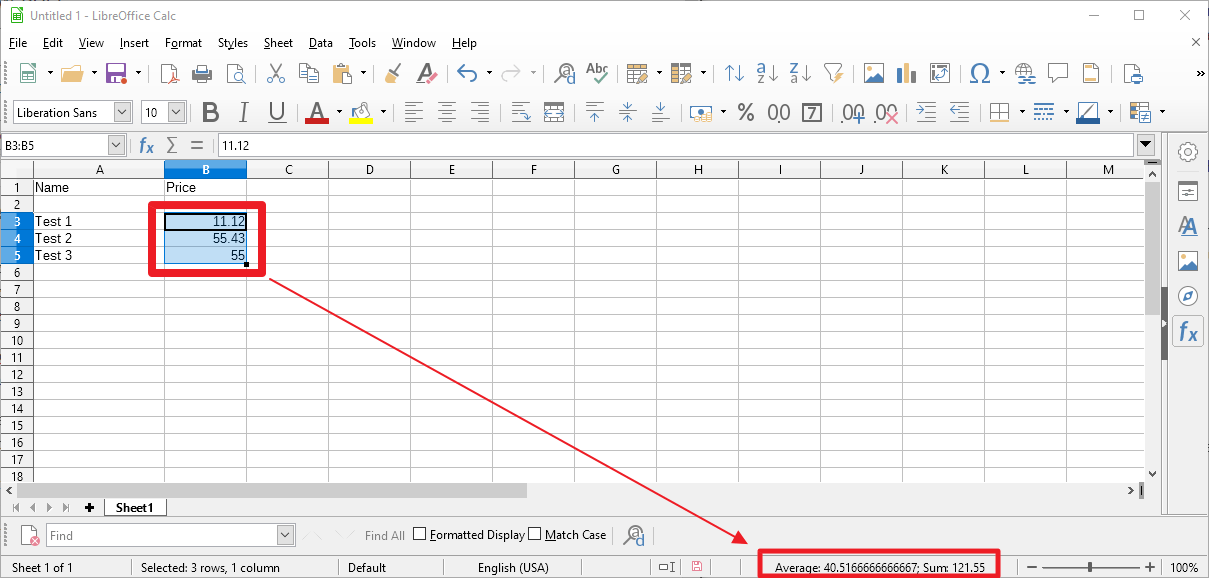
6. Utilize the status bar: The status bar at the bottom of the Calc window provides helpful information about selected cells, including the sum. Simply highlight the range, and the sum will appear in the status bar.

7. Sort your data: Before adding up columns or rows, consider sorting the data to group similar values together. This can make it easier to identify patterns and ensure accurate calculations.

8. Use autofilter: Applying autofilter allows you to filter out specific values or criteria and then calculate the sum of the visible cells only. This can be helpful when working with large datasets that require selective calculations.

By implementing these tips and tricks, you can streamline your workflow and perform calculations more efficiently in Open Office Calc. These techniques will enhance your productivity and accuracy when adding up columns or rows of numbers in your spreadsheets.