Open Office Calc Basic Spreadsheet Tutorial

Defining Spreadsheets

A spreadsheet is a powerful tool used to organize and analyze data in a structured manner. It consists of rows and columns, forming a grid-like structure where cells are created at their intersection. Spreadsheets are commonly used in various fields, including finance, accounting, project management, and data analysis.

At its core, a spreadsheet provides a flexible environment for storing and managing numerical data. It allows you to enter, manipulate, and perform calculations on the data within the cells. With its functionality, you can easily perform mathematical operations such as addition, subtraction, multiplication, and division, making it an essential tool for handling numerical information.

What sets spreadsheets apart from other data storage solutions is its formula capability. You can create formulas that automatically calculate values based on the data in other cells. This feature is especially useful when dealing with complex calculations or when working with large datasets.

Spreadsheets also offer the ability to format data, making it easier to read and understand. You can apply different formats to cells, including number formats, currency formats, date formats, and more. Additionally, you can customize the appearance of the spreadsheet by changing font styles, colors, and applying conditional formatting rules.

Collaboration is another key aspect of spreadsheets. With cloud-based spreadsheet software, multiple users can work on the same spreadsheet simultaneously, making it a collaborative tool for teams. This allows for real-time updates and enables efficient teamwork, especially when dealing with complex projects or shared data analysis.

Overall, spreadsheets provide a versatile platform for managing and analyzing data. Their flexibility, formula capability, and formatting options make them an invaluable tool for businesses and individuals alike. Whether you need to track expenses, create budget plans, or analyze sales data, spreadsheets can simplify and streamline these tasks, allowing you to make informed decisions based on organized and accurate information.

Navigating the Open Office Calc Interface

Open Office Calc, a part of the Open Office suite, provides a user-friendly interface for creating and managing spreadsheets. Familiarizing yourself with the interface will help you navigate through the various features and tools available, allowing you to work efficiently and effectively.

Upon opening Open Office Calc, you will be presented with a blank spreadsheet, also known as a workbook. The interface consists of several key elements:

Menu Bar: Located at the top of the application, the menu bar contains various menus such as File, Edit, View, and Format. These menus provide access to a wide range of commands and options for customizing your spreadsheet.
Toolbar: Directly below the menu bar, the toolbar contains icons representing frequently used commands. It provides quick access to common functions such as saving, formatting, and inserting data.
Formula Bar: Situated below the toolbar, the formula bar displays the contents of the currently selected cell. It allows you to enter and edit cell data, including formulas and functions.
Column Headers: Located above the spreadsheet grid, the column headers are labeled with letters from A to Z and beyond. These headers represent the columns in the spreadsheet, allowing you to easily identify and navigate to specific columns.
Row Headers: Situated on the left side of the spreadsheet grid, the row headers are numbered from 1 onwards. These headers represent the rows in the spreadsheet, providing a convenient way to locate and access specific rows.
Spreadsheet Grid: The main area of the interface is occupied by the spreadsheet grid. It consists of cells organized in rows and columns. You can enter and manipulate data within these cells, perform calculations, and apply various formatting options.
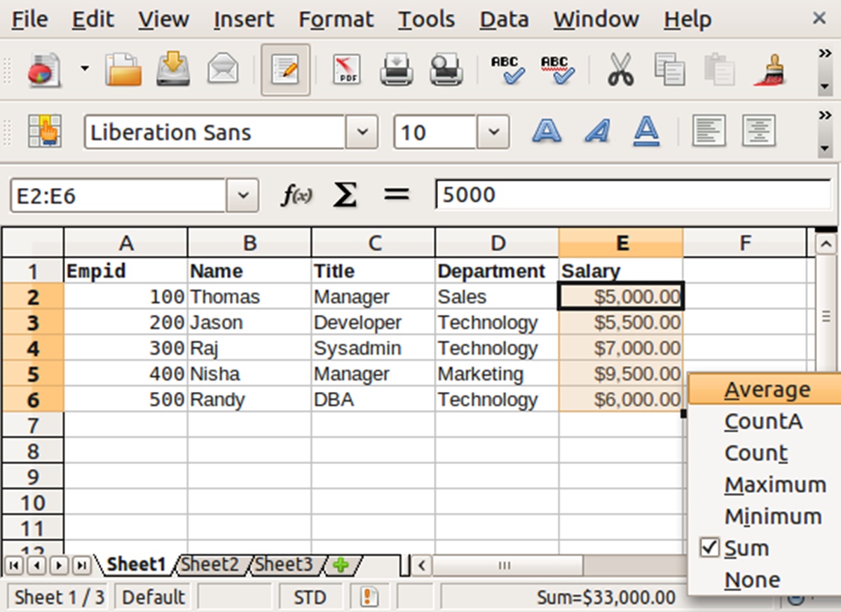
Status Bar: Located at the bottom of the application, the status bar displays useful information such as the current cell’s coordinates, the sum of selected cells, and the status of various functions such as AutoFill and AutoCalculate.

By understanding and utilizing these interface elements, you can efficiently navigate through your spreadsheet, access important commands and functions, and make the most out of Open Office Calc’s powerful features. Taking the time to familiarize yourself with the interface will greatly enhance your productivity and allow you to create and manage spreadsheets with ease.

Creating a New Spreadsheet

Open Office Calc makes it quick and easy to create a new spreadsheet to start organizing your data. Follow these simple steps to create a new spreadsheet:

Open Open Office Calc by clicking on the application icon or by selecting it from the Start menu.
Once Open Office Calc is open, you will be presented with a blank spreadsheet.
Start entering your data into the cells of the spreadsheet. You can navigate to different cells using the arrow keys or by simply clicking on the desired cell.
To add more rows or columns, right-click on the row or column headings and select “Insert Rows” or “Insert Columns” from the context menu.
To save your spreadsheet, click on the “File” menu at the top-left corner of the interface and select “Save” or use the shortcut Ctrl + S. Choose a location and provide a name for your spreadsheet, then click “Save”.
If you want to create a new spreadsheet based on a template, you can select the desired template from the “File” menu by choosing “New” and selecting from the available templates.
To open an existing spreadsheet, go to the “File” menu and select “Open”. Browse to the location where your spreadsheet is saved, select it, and click “Open”.

When creating a new spreadsheet, it’s important to consider the structure and layout of your data. Define the columns and rows based on the type of data you will be entering. Properly labeling and formatting cells can greatly enhance the readability and organization of your spreadsheet.

Remember to save your spreadsheet regularly to avoid losing any valuable data. Additionally, consider using different sheets within a workbook to organize related data and keep your spreadsheets well-structured.

Creating a new spreadsheet in Open Office Calc is a straightforward process that allows you to quickly begin organizing and analyzing your data. By following these steps and taking advantage of the various features and tools available, you can efficiently create and manage your spreadsheets for personal or professional use.

Saving and Opening Spreadsheets

One of the fundamental tasks when working with spreadsheets is saving and opening them to ensure your data is securely stored and easily accessible. Open Office Calc provides a simple and convenient way to save and open spreadsheets. Here’s how:

To save a spreadsheet, click on the “File” menu at the top-left corner of the interface and select “Save” or use the shortcut Ctrl + S. Choose a location on your computer where you want to save the spreadsheet and provide a name for it. Then click “Save”.
If you want to save a copy of the spreadsheet in a different file format, such as Microsoft Excel or PDF, select “Save As” from the “File” menu. Choose the desired file format from the drop-down menu and click “Save”.
To open an existing spreadsheet, go to the “File” menu and select “Open”. Browse to the location where your spreadsheet is saved, select it, and click “Open”. Alternatively, you can use the shortcut Ctrl + O to open the “Open” dialog box.
If you frequently work on the same set of spreadsheets, you can create shortcuts to them by using the “Recent Documents” list found in the “File” menu. This allows you to quickly access your most-used spreadsheets without having to navigate to their saved locations.
Open Office Calc also provides auto-saving functionality. By default, it automatically saves your spreadsheet every 10 minutes. You can adjust the auto-save frequency or disable it altogether by going to the “Tools” menu and selecting “Options”. From there, navigate to the “Load/Save” section and choose “General”. Here, you can modify the auto-save settings according to your preferences.
When opening a spreadsheet, Open Office Calc will display it in a new window. You can have multiple spreadsheets open simultaneously and switch between them using the tabs at the bottom of the interface.

Saving your spreadsheets regularly is crucial to avoid losing important data. It is recommended to establish a backup routine to further protect your spreadsheets from accidental loss or system failures. You can create backups by manually copying your saved spreadsheets to an external storage device or utilizing automatic backup software.

By mastering the methods for saving and opening spreadsheets in Open Office Calc, you can ensure the security and accessibility of your data and streamline your workflow for efficient spreadsheet management.

Understanding Rows, Columns, and Cells

In Open Office Calc, understanding the basic elements of a spreadsheet, such as rows, columns, and cells, is essential for efficient data organization and manipulation. Each of these components plays a vital role in structuring and managing your spreadsheet:

Rows: Rows are horizontal lines in a spreadsheet, numbered sequentially from the top. They allow you to organize and categorize your data horizontally. Each row is identified by its number and contains individual cells where data can be entered.
Columns: Columns are vertical lines in a spreadsheet, labeled alphabetically from left to right. They enable you to categorize and organize data vertically. Each column is identified by its letter and contains individual cells for data entry.
Cells: Cells are the building blocks of a spreadsheet, created at the intersection of rows and columns. They are the individual units where you can input and manipulate data. Each cell is identified by its unique combination of a column letter and a row number.

Cells are the core components of a spreadsheet and are used to store various types of data, including numbers, text, dates, and formulas. They can be formatted to display the data in different ways, such as currency formatting, percentage formatting, or as a date. Cells can also be given specific alignment, font styles, and background colors to enhance the visual presentation of your data.

Rows and columns provide the structure for organizing your data. They allow you to classify information into logical groups and make it easier to navigate and analyze. For example, in a sales spreadsheet, you might have columns for product names, quantities sold, and sales prices, while each row represents a specific sale entry.

To select a row or column in Open Office Calc, simply click on its corresponding row header or column header. You can select multiple rows or columns by holding down the Shift key and clicking on the desired headers. This allows you to perform actions on multiple cells simultaneously, such as formatting, deleting, or copying data.

Understanding the relationship between rows, columns, and cells is crucial for effective spreadsheet management. Organizing your data into rows and columns helps maintain a structured and coherent spreadsheet, making it easier to analyze, sort, and filter the data as needed.

By making full use of the grid-like structure provided by rows, columns, and cells, Open Office Calc simplifies the process of data entry, organization, and manipulation, allowing you to create powerful and informative spreadsheets.

Entering and Editing Data in Cells

Entering and editing data in cells is a fundamental task when working with spreadsheets. Open Office Calc provides various tools and techniques to effortlessly input and modify data in your spreadsheet:

Entering Data: To enter data into a cell, simply click on the desired cell and start typing. You can enter numbers, text, dates, or formulas. Pressing the Enter key or moving to another cell confirms the data entry. If you want to edit the data you just entered, double-click on the cell to activate edit mode.
Copying and Pasting Data: You can quickly copy and paste data in Open Office Calc. To copy data from one cell to another, select the cell, click on the “Edit” menu, and choose “Copy” or use the shortcut Ctrl + C. Then, select the target cell and click on the “Edit” menu, selecting “Paste” or using the shortcut Ctrl + V to paste the copied data.
Moving Data: If you want to move data to another location within the spreadsheet, select the cell or range of cells you wish to move, click and hold the selection, and drag it to the desired location. Release the mouse button to complete the move operation.
Deleting Data: To delete data from a cell or a range of cells, select the cell(s) containing the data, click on the “Edit” menu, and choose “Delete Cells” or use the shortcut Ctrl + -, then select the desired deletion options and click “OK”.
Automatic Calculations: Open Office Calc has built-in functionality for automatic calculations. You can input simple calculations directly into cells by using arithmetic operators (+, -, *, /) and cell references (e.g., A1, B2). The calculated result will automatically update when the input values change.
Editing Data: To edit data in a cell, double-click on the cell to activate edit mode and make the necessary changes. Press Enter or move to another cell to confirm the edited data. Alternatively, you can also click on the cell once and directly modify the data in the formula bar located at the top of the interface.

When entering and editing data, it is important to ensure accuracy and correctness. Open Office Calc provides validation options to help you validate data entry, such as setting up data limits, applying data validation rules, or utilizing the spelling checker.

By utilizing these features and techniques, you can efficiently enter and edit data in cells, ensuring the accuracy and integrity of your spreadsheet. Whether you are working with simple numbers or complex formulas, Open Office Calc provides the tools you need to effectively manage and manipulate data within your spreadsheet.

Formatting Cells, Rows, and Columns

Open Office Calc provides a wide range of formatting options to enhance the appearance and readability of your spreadsheet. With formatting, you can customize the font style, apply colors, change cell borders, and much more. Here’s how you can format cells, rows, and columns:

Cell Formatting: To format a single cell, select the desired cell and right-click to open the context menu. From the menu, choose “Format Cells” to access the formatting options. Here you can change the number format, apply font styles, adjust alignment, and modify other cell-specific formatting settings.
Row and Column Formatting: To format an entire row or column, right-click on the row or column header and select “Format Cells”. This allows you to apply formatting options to the entire row or column, including number formatting, font styles, alignment, and more. You can also adjust the width of columns or the height of rows by clicking and dragging the borders between the headers.
Conditional Formatting: Open Office Calc provides conditional formatting options that allow you to automatically format cells based on specific conditions. To apply conditional formatting, select the range of cells you want to format, click on the “Format” menu, choose “Conditional Formatting”, and set the desired formatting rules based on values, formulas, or other criteria.
Cell Styles: Cell styles enable you to apply predefined formatting combinations quickly. Open Office Calc offers a variety of built-in cell styles to choose from, such as Title, Heading, Currency, and more. To apply a cell style, select the desired cells, click on the “Format” menu, choose “Styles and Formatting”, and select the appropriate cell style from the sidebar.
Merging Cells: You can merge cells in Open Office Calc to create a single larger cell. This is useful when you want to highlight a title or create a visually appealing layout. To merge cells, select the cells you wish to merge, right-click to open the context menu, and choose “Merge Cells”.

Formatting cells, rows, and columns not only improves the visual appearance of your spreadsheet but also helps to organize and present your data more effectively. By applying consistent formatting techniques, you can enhance readability and make your spreadsheet more professional and visually appealing.

Experiment with various formatting options provided by Open Office Calc to find the styles and combinations that work best for your specific needs. Whether you’re creating a financial report, a project timeline, or a data analysis sheet, proper cell, row, and column formatting can greatly enhance the functionality and presentation of your spreadsheet.

Inserting and Deleting Rows and Columns

Open Office Calc allows you to easily insert and delete rows and columns to modify the structure and layout of your spreadsheet. These actions can help you reorganize data, accommodate additional information, or remove unnecessary elements. Here’s how you can insert and delete rows and columns:

Inserting Rows: To insert a new row, right-click on the row header above which you want to insert the row. From the context menu, select “Insert Rows”. A new row will be added above the selected row, shifting the existing rows down.
Inserting Columns: To insert a new column, right-click on the column header to the left of which you want to insert the column. From the context menu, select “Insert Columns”. A new column will be added to the left of the selected column, pushing the existing columns to the right.
Deleting Rows: To delete a row, right-click on the row header of the row you want to delete and select “Delete Rows” from the context menu. The selected row will be deleted, and the remaining rows will shift up to fill the gap.
Deleting Columns: To delete a column, right-click on the column header of the column you want to delete and choose “Delete Columns” from the context menu. The selected column will be deleted, causing the remaining columns to shift to the left.
Keyboard Shortcuts: You can also use keyboard shortcuts to insert and delete rows and columns. For inserting rows, use the shortcut Ctrl + Shift + + (plus key). To insert columns, employ the shortcut Ctrl + Shift + – (minus key). For deleting rows, press Shift + Space to select the entire row and then use the shortcut Ctrl + – (minus key). To delete columns, select the entire column and use the shortcut Ctrl + – (minus key).

Inserting rows and columns allows you to expand your spreadsheet without disrupting the existing data or formatting. It enables you to add new information or adjust the layout to accommodate changes in your data requirements.

On the other hand, deleting rows and columns helps in removing unnecessary data or adjusting the structure of your spreadsheet. This allows you to maintain a clean and organized layout.

By utilizing the techniques for inserting and deleting rows and columns in Open Office Calc, you have the flexibility to adapt your spreadsheet to changing data needs, ensuring its effectiveness and efficiency for data management and analysis.

AutoFill and AutoComplete Features

Open Office Calc comes equipped with powerful AutoFill and AutoComplete features that can save you time and simplify data entry tasks. These features automatically fill in data or suggest entries based on existing patterns or previously entered values. Both AutoFill and AutoComplete provide efficient ways to enter data and maintain consistency in your spreadsheet:

AutoFill: AutoFill allows you to quickly populate a series of cells with a pattern or sequence. For example, if you enter a number or text in a cell and drag the fill handle (a small square at the bottom-right corner of the selected cell), Open Office Calc will automatically fill in the adjacent cells with a continuation of the series. AutoFill recognizes patterns in data, such as dates, months, days of the week, or numerical sequences, making it effortless to populate a column or row with consistent data.
AutoComplete: AutoComplete suggests entries based on previously entered values in the same column. As you begin typing in a cell, Calc looks for matching entries in the column and displays a dropdown list of suggestions. Using the arrow keys or the mouse, you can choose the desired value from the suggestions, and Calc will automatically complete the cell entry. This is particularly helpful when entering repetitive or frequently used values, saving time and minimizing errors.
Custom AutoFill Lists: Open Office Calc allows you to create custom AutoFill lists. This feature is beneficial when you have a specific set of data that you want to repeatedly enter into cells. To create a custom AutoFill list, go to the “Tools” menu, select “Options”, choose the “Open Office Calc” category, and click on the “Custom Lists” tab. Here, you can define your custom list and then use AutoFill to quickly populate cells with those values.
AutoFill Options: Open Office Calc provides several options for controlling AutoFill behavior. You can access these options by going to the “Tools” menu, selecting “Options”, and navigating to the “Open Office Calc” category. Under the “General” tab, you can customize the AutoFill settings, such as enabling or disabling AutoFill, modifying the direction of the filled series, or changing the behavior when copying cells with formulas.

By leveraging the AutoFill and AutoComplete features, you can significantly speed up data entry and maintain consistency in your spreadsheet. These features not only save you time but also help prevent data entry errors and ensure accuracy in your calculations and analyses. Take advantage of these powerful tools provided by Open Office Calc to streamline your workflow and enhance productivity.

Creating Simple Formulas

Open Office Calc allows you to perform calculations on your spreadsheet data by creating and using simple formulas. Formulas are expressions that combine numbers, operators, and cell references to produce calculated results. Here’s how you can create simple formulas in Open Office Calc:

Select the cell where you want the result of your formula to appear.
Start the formula by typing the equals sign “=” in the selected cell. This tells Calc that you are entering a formula.
Enter the formula using appropriate operators, such as “+”, “-“, “*”, and “/”. You can use cell references instead of values to include data from other cells in your calculations. For example, entering “=A1+B1” in a cell will add the values from cells A1 and B1.
To include cell references in your formula, you can either type them directly or select the desired cells with the mouse. Calc will automatically insert the cell reference into the formula for you.
Press Enter to confirm and execute the formula. The result will be displayed in the cell where you entered the formula.

Formulas can be as simple or as complex as needed, depending on the desired calculations. You can perform a wide range of mathematical operations, such as addition, subtraction, multiplication, and division, using cell references or constant values.

Open Office Calc also supports various functions that you can use in your formulas, such as SUM, AVERAGE, MAX, MIN, and COUNT. These built-in functions offer specialized calculations that can simplify and enhance your data analysis tasks.

When creating formulas, it’s important to properly use parentheses to control the order of operations. Calc follows the standard mathematical precedence, calculating operations within parentheses first, and then performing other operations from left to right.

In addition, Open Office Calc provides error-checking capabilities that alert you to potential formula errors. If Calc detects an issue with your formula, it will display an error message in the cell, helping you identify and correct the problem.

By mastering the skill of creating simple formulas in Open Office Calc, you can perform efficient calculations and manipulate your spreadsheet data effectively. Formulas allow you to automate calculations, saving time and effort while ensuring accurate results.

Understanding Functions and Formulas

In Open Office Calc, functions and formulas are powerful tools that enable you to perform complex calculations and manipulate data in your spreadsheet. Understanding how functions and formulas work can greatly enhance your ability to analyze and process data effectively:

Functions:

A function is a predefined formula that performs specific calculations or manipulations on data. Open Office Calc provides a wide range of built-in functions that you can use to perform common mathematical and statistical operations, manipulate text, work with dates and times, and more.

Functions are typically written as a word followed by parentheses. The data or values that need to be processed are placed within the parentheses, separated by commas if necessary. For example, the SUM function adds up a range of numbers and is written as “SUM(A1:A10)”, where A1:A10 represents the range of cells to be summed.

Using functions allows you to perform complex calculations with ease and efficiency. Functions help to streamline your calculations and eliminate the need for long and complicated formulas.

Formulas:

A formula is an expression that combines values, cell references, and functions to perform calculations or operations in a spreadsheet. Formulas are entered into cells and are usually preceded by an equals sign (=) to indicate that it is a formula.

Formulas can be as simple as adding two numbers together or as complex as performing multiple calculations using various functions. They can also refer to cells in other sheets within the same workbook.

When creating formulas, you can use arithmetic operators (+, -, *, /) to perform basic mathematical operations, as well as parentheses to control the order of operations. You can also use cell references to include data from other cells in your formulas.

Understanding how functions and formulas work together allows you to leverage the full potential of Open Office Calc. By using functions, you can perform specialized calculations and operations on your data, while formulas allow you to customize and tailor calculations to meet your specific needs.

Take the time to explore the wide range of functions available in Open Office Calc and experiment with different formulas. This will enable you to analyze and manipulate your data more effectively, leading to enhanced insights and productivity.

Using Built-in Functions in Open Office Calc

Open Office Calc provides a vast array of built-in functions that can greatly simplify and enhance your data analysis tasks. These functions perform a wide range of calculations, statistical analysis, text manipulation, date and time operations, and more. Understanding how to use built-in functions can significantly streamline your spreadsheet work:

Syntax and Arguments:

Each function in Open Office Calc has a specific syntax, which includes the function name followed by parentheses. Within the parentheses, you provide the necessary arguments or inputs for the function to operate on. These arguments can be values, cell references, or other functions.

For example, the SUM function is widely used to calculate the sum of a range of values. The syntax for the SUM function is “=SUM(argument1, argument2, …)”, where the arguments represent the cells or values to be summed. The function may take multiple arguments, separated by commas.

Using Functions:

To use a built-in function in Open Office Calc, follow these steps:

Select the cell where you want the result of the function to appear.
Begin typing the function name, or click on the “Insert Function” button (represented by the fx symbol) on the Formula Bar.
As you type or select the function, Calc will provide a description of the function and its arguments.
Enter the necessary arguments within the parentheses, either by typing directly or selecting cells or ranges with the mouse.
Press Enter to execute the function and display the result in the selected cell.

Commonly Used Functions:

Open Office Calc offers a vast selection of built-in functions. Some commonly used functions include:

SUM: Calculates the sum of a range of values.
AVERAGE: Calculates the average of a range of values.
MAX: Returns the maximum value from a range.
MIN: Returns the minimum value from a range.
IF: Performs a conditional test and returns different values based on the result.
CONCATENATE: Joins multiple text strings together.
DATE: Creates a date using specified year, month, and day values.
NOW: Returns the current date and time.

These commonly used functions are just a glimpse of the immense functionality provided by Open Office Calc. By exploring the available functions and their capabilities, you can unleash the full potential of your spreadsheet and perform complex calculations and analyses with ease.

Utilizing built-in functions allows you to automate repetitive tasks, save time, and ensure accuracy in your data analysis. Experiment with different functions and explore their capabilities to enhance your spreadsheet work.

Formatting Spreadsheet Data

Formatting plays a vital role in making your spreadsheet data more visually appealing, organized, and easier to read. Open Office Calc provides numerous formatting options to help you customize the appearance of your spreadsheet. Here’s how you can format your spreadsheet data:

Number Formatting:

You can apply specific number formats to cells in Open Office Calc to display numerical values in different ways. For example, you can format a cell to display numbers as currency, percentages, dates, or scientific notation. To apply number formatting, select the desired cells, right-click, and choose “Format Cells”. In the Format Cells dialog box, navigate to the “Numbers” category and choose the desired number format.

Font Formatting:

Customizing the font style, size, and color can significantly improve the readability and aesthetics of your spreadsheet. You can modify the font formatting by selecting the cells you want to format, right-clicking, and choosing “Format Cells”. In the Format Cells dialog box, navigate to the “Font” category to adjust various font settings such as font style, size, color, and text effects.

Alignment and Wrapping:

Adjusting cell alignment allows you to control how the contents of a cell are positioned within the cell. Open Office Calc provides options to align text horizontally (left, center, or right), vertically (top, middle, or bottom), or justify text. You can also wrap the text within a cell to display all the contents without truncation. To modify text alignment and wrapping, select the cells you want to format, right-click, and choose “Format Cells”. In the Format Cells dialog box, navigate to the “Alignment” category to adjust the alignment and wrapping settings.

Conditional Formatting:

Conditional formatting allows you to automatically apply formatting to cells based on specific conditions or criteria. This feature is handy for highlighting important data, identifying trends, or emphasizing exceptional values. To apply conditional formatting, select the cells to format, click on the “Format” menu, choose “Conditional Formatting”, and set up the desired formatting rules based on values, formulas, or other criteria.

Cell Borders and Fill Colors:

You can enhance the visual appeal and organization of your spreadsheet by applying cell borders and fill colors. Borders help differentiate cells and create clearer cell boundaries, while fill colors allow you to highlight specific cells or ranges. To add borders or apply fill colors, select the cells you want to format, right-click, and choose “Format Cells”. In the Format Cells dialog box, navigate to the “Border” or “Background” categories to adjust the border and fill color settings.

By effectively utilizing formatting options offered by Open Office Calc, you can transform your spreadsheet into a professional and visually appealing document. Take the time to experiment with different formatting techniques and find the style that best suits your data and presentation needs.

Using Conditional Formatting

Conditional formatting is a powerful feature in Open Office Calc that allows you to apply formatting to cells based on specific conditions or criteria. This feature can help you highlight important data, identify patterns, and visualize trends within your spreadsheet. Here’s how you can use conditional formatting:

Select the cells or range of cells that you want to apply conditional formatting to.
Click on the “Format” menu at the top of the interface and choose “Conditional Formatting” from the drop-down menu.
The conditional formatting dialog box will appear, presenting you with a range of formatting options to choose from.
Specify the criteria or conditions that should trigger the formatting. This can include numerical comparisons, text matches, date ranges, or custom formulas.
Choose the formatting style you want to apply when the specified condition is met. This can include font styles, background colors, borders, and more.
Preview the formatting to ensure it looks as desired, and make any additional adjustments as needed.
Click “OK” to apply the conditional formatting to the selected cells.

Conditional formatting opens up a world of possibilities for data visualization. You can use it to highlight cells that meet certain criteria, such as values above a certain threshold, duplicates, or errors. You can also create color scales or data bars to show the relative values of cells within a range.

Furthermore, conditional formatting is not limited to single cells or ranges. You can apply it to entire rows or columns, making it easier to spot trends or patterns in your data.

By effectively using conditional formatting, you can quickly identify outliers, visualize data relationships, and make your spreadsheet more visually informative. It is a valuable tool for data analysis, allowing you to draw attention to specific cells or ranges based on user-defined criteria.

Take the time to explore the various conditional formatting options provided by Open Office Calc, and unleash the potential of visualizing your data in meaningful ways.

Sorting and Filtering Data

Open Office Calc provides powerful tools for sorting and filtering data in your spreadsheet. Sorting allows you to arrange data in a specific order, while filtering enables you to display only the data that meets certain criteria. These features make it easier to analyze and extract information from your dataset. Here’s how you can use sorting and filtering in Open Office Calc:

Sorting Data:

To sort data in Open Office Calc, follow these steps:

Select the range of cells that you want to sort.
Click on the “Data” menu at the top of the interface and choose “Sort” from the drop-down menu.
In the Sort dialog box, select the column or columns that you want to use for sorting. You can specify the sorting order, such as ascending or descending.
Click “OK” to apply the sorting to the selected cells. The data will be rearranged based on the specified criteria.

Sorting data allows you to organize your dataset based on specific columns or criteria. It can be helpful for arranging data in alphabetical order, numerical order, or based on other factors such as dates or custom defined order.

Filtering Data:

To filter data in Open Office Calc, follow these steps:

Select the range of cells that you want to filter.
Click on the “Data” menu at the top of the interface and choose “Filter” from the drop-down menu.
AutoFilter arrows will appear in the header row of each column. Click on the arrow of the column you want to filter.
In the dropdown menu, select the desired criteria or values to filter by. You can apply multiple filters to different columns to further refine the results.
The displayed data will be filtered based on the selected criteria. You can also use custom filter options to create more complex filtering conditions.

Filtering data allows you to focus on specific subsets of your dataset that meet certain criteria. This can be useful for analyzing specific data ranges, identifying unique values, or finding specific patterns within your data.

By effectively using sorting and filtering in Open Office Calc, you can quickly organize and analyze your data, extract valuable insights, and make informed decisions based on the filtered or sorted results.

Take advantage of these powerful tools to streamline your data analysis tasks and make the most out of your spreadsheet data.

Creating Charts and Graphs from Spreadsheet Data

Open Office Calc offers robust charting capabilities that allow you to visually represent your spreadsheet data in the form of charts and graphs. Charts provide a powerful way to communicate information, identify trends, and highlight patterns within your data. Here’s how you can create charts and graphs in Open Office Calc:

Select the range of cells that you want to include in your chart. This range should contain both the data and the labels you want to represent.
Click on the “Insert” menu at the top of the interface and choose “Chart” from the drop-down menu.
The Chart Wizard will appear, presenting you with a selection of chart types to choose from, such as bar charts, line charts, pie charts, and more.
Select the desired chart type that best suits your data. You can preview each chart type before finalizing your selection.
Specify the range of data to be used for the chart by selecting the appropriate cells or by manually entering the cell references.
Customize the chart elements, including titles, axis labels, colors, legends, and other formatting options, as per your preferences.
Preview the chart to ensure it accurately represents your data and presents it in a clear and visually appealing manner.
Click “Finish” to create the chart. It will be inserted into your spreadsheet as a dynamic object that can be resized and moved as needed.

Charts provide a visual representation of your data, making it easier to interpret and analyze. They allow you to identify trends, compare values, and spot patterns within your dataset.

Additionally, Open Office Calc provides options to further enhance and customize your charts. You can add data labels, adjust the axis scales and formatting, apply different chart styles, and even combine multiple chart types in a single chart to visualize complex relationships.

By creating charts and graphs in Open Office Calc, you can effectively communicate your data to others, make data-driven decisions, and present your findings in a visually compelling way.

Experiment with different chart types and formatting options to find the best representation for your data, and utilize the power of charts to unlock deeper insights from your spreadsheet information.

Printing Spreadsheets

Open Office Calc provides a range of options and settings to help you print your spreadsheets efficiently and effectively. Whether you need a physical copy for reference or to share your data with others, here’s how you can print your spreadsheets:

Open the spreadsheet that you want to print in Open Office Calc.
Click on the “File” menu at the top-left corner of the interface and select “Print” or use the shortcut Ctrl + P.
In the Print dialog box, you can customize various settings to meet your printing requirements:

Printer Selection: Choose the printer you want to use from the available options.
Page Range: Specify the pages or range of pages you want to print. Options include printing the entire spreadsheet, current sheet, or selecting specific page ranges.
Page Layout: Adjust the page orientation (portrait or landscape), paper size, margins, and other settings to ensure the spreadsheet fits neatly on the printed page.
Scaling: You can scale the spreadsheet to fit the pages by adjusting the scaling options. This ensures that the data is legible and well-formatted when printed.

Preview the printout using the “Preview” button to ensure that the printed version appears as you desire.
Once you are satisfied with the print settings, click “Print” to send the spreadsheet to the selected printer.

When printing spreadsheets, it is crucial to consider the layout and formatting to ensure that the information is presented clearly and accurately. Adjusting the page orientation, margins, and scaling can help optimize the printout.

You can also set print areas to define specific sections of the spreadsheet that you want to print. To set a print area, select the desired cells or range of cells, click on the “Format” menu, choose “Print Ranges”, and select “Define” to set the print area.

Moreover, Open Office Calc provides the option to print gridlines and headings, making it easier to read and navigate the printed spreadsheet.

By utilizing the printing capabilities of Open Office Calc, you can effectively share and distribute your spreadsheet data in a physical format. Take advantage of the various customization options to tailor the printout to your specific needs.

Importing and Exporting Data

Open Office Calc provides convenient features for importing and exporting data, allowing you to work seamlessly with data from various sources and share your spreadsheet information with others. Here’s how you can import and export data in Open Office Calc:

Importing Data:

To import data into Open Office Calc, follow these steps:

Click on the “File” menu at the top-left corner of the interface and select “Open” or use the shortcut Ctrl + O.
In the Open dialog box, navigate to the location of the data file you want to import.
Select the file and click “Open”.
The “Text Import” dialog box will appear, allowing you to specify how you want to import the data. Choose the file type, delimiter, and other settings according to the structure of the imported data.
Preview the imported data to ensure it appears as expected.
Click “OK” to import the data into Open Office Calc, where you can further manipulate and analyze it.

Open Office Calc supports a wide range of file formats for importing data, including CSV, XLSX, and ODS, among others. This flexibility allows you to integrate data from different sources seamlessly.

Exporting Data:

To export data from Open Office Calc, follow these steps:

Click on the “File” menu at the top-left corner of the interface and select “Save As”.
In the Save As dialog box, choose the desired file format for export from the available options, such as XLSX, CSV, or PDF.
Specify the location where you want to save the exported file and provide a name for it.
Click “Save” to export the data from Open Office Calc in the selected file format.

Exporting data allows you to share your spreadsheet information with others who may not have Open Office Calc or need the data in a different format. It also helps in creating backups or archiving data.

In addition to exporting entire spreadsheets, you can export specific ranges or sheets by selecting the desired cells or sheets before initiating the export process.

By leveraging the importing and exporting features of Open Office Calc, you can seamlessly integrate data from various sources, collaborate with others using different software applications, and easily share your spreadsheet information in a format that suits your needs.

Tips and Tricks for Efficient Spreadsheet Usage

Mastering the efficient usage of spreadsheets can greatly enhance your productivity and make working with data more streamlined. Here are some helpful tips and tricks to optimize your experience with Open Office Calc:

Use keyboard shortcuts: Memorize and utilize keyboard shortcuts to perform common tasks quickly. For example, Ctrl + S to save, Ctrl + C to copy, Ctrl + V to paste, and Ctrl + Z to undo.
Freeze panes: Freeze rows or columns to keep essential information visible while scrolling through large datasets. Go to the “Window” menu, choose “Freeze”, and select the desired rows or columns to freeze.
Create named ranges: Define named ranges for specific cells or cell ranges to refer to them easily in formulas. This allows for more readable and maintainable formulas.
Use data validation: Apply data validation rules to ensure data integrity and prevent errors. Go to the “Data” menu, choose “Validity”, and set criteria such as numerical limits, text length, or custom formulas for input validation.
Utilize conditional formatting: Apply conditional formatting to highlight specific cells or ranges based on predefined criteria. This helps draw attention to important data patterns or outliers.
Get familiar with functions: Take time to explore and understand the wide range of built-in functions available in Open Office Calc. Utilize them to perform various calculations, statistical analyses, and data manipulations.
Organize data with sheets: Use multiple sheets within a single workbook to separate and organize related data sets. Rename and color-code sheets for easier navigation.
Back up your data: Regularly save copies of your spreadsheet to ensure data safety. Consider utilizing cloud storage or external backups for added protection against data loss.
Document your spreadsheet: Add comments and documentation to clarify complex formulas or provide additional context. This helps make your spreadsheet more understandable for yourself and others.
Collaborate with others: Make use of cloud-based storage platforms and collaboration tools to enable real-time collaboration and efficient teamwork on spreadsheets.

By incorporating these tips and tricks into your spreadsheet usage, you can save time, enhance data accuracy, and improve overall efficiency. Experiment with new features, explore additional functionalities, and find the best practices that work for you and your specific spreadsheet needs.