
What is the Excel INDEX function?
The INDEX function in Excel is a powerful tool that allows you to retrieve data from a specific row and column within a range or array. It is commonly used in formulas to dynamically extract information based on certain criteria or conditions. With the INDEX function, you can avoid manual search and lookup operations, saving both time and effort.
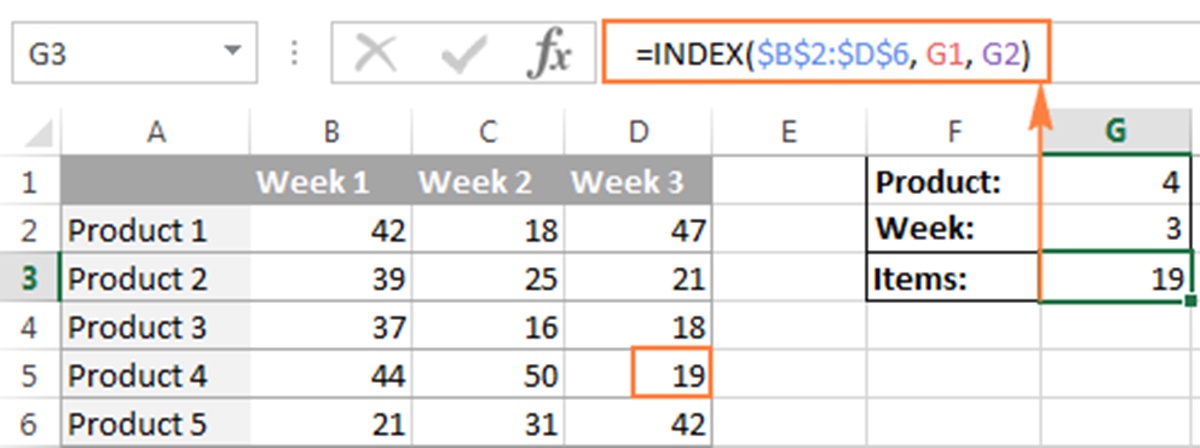
At its core, the INDEX function takes two main arguments: the array and the row or column number. The array can be a range of cells or an array constant, and the row or column number specifies the location from which you want to extract the data.
For example, if you have a table of sales data with multiple rows and columns, you can use the INDEX function to retrieve the value at a specific intersection point, such as the sales amount for a particular product and month.
The INDEX function can be further enhanced by combining it with other functions like MATCH, which allows you to find the position of a specific value within an array. This dynamic combination is especially useful when working with large datasets or complex data structures.
One of the key benefits of using the INDEX function is its versatility. You can use it in various scenarios, including creating dynamic reports, generating summaries, and performing complex calculations. Whether you need to retrieve data from a single table or multiple tables, the INDEX function can handle different data types and return the desired results efficiently.
Overall, the Excel INDEX function is an essential tool in data analysis and manipulation. It provides a flexible and efficient way to extract data from arrays or ranges, making it easier to work with large datasets and automate repetitive tasks. Understanding how to use the INDEX function can significantly improve your productivity and effectiveness in Excel.
Syntax of the INDEX function
The INDEX function in Excel follows a specific syntax that determines the arguments it accepts and how they should be formatted. Understanding the syntax is crucial for effectively using the INDEX function in your formulas. The basic syntax of the INDEX function is:
=INDEX(array, row_num, [column_num])
Let’s break down each component of the syntax:
- Array: This is the range or array from which you want to extract data. It can be a single range, a named range, or an array constant.
- Row_num: This parameter specifies which row within the array you want to retrieve data from. It accepts a numeric value or a cell reference.
- Column_num: This optional parameter is used when the array has multiple columns. It specifies the column from which you want to retrieve data. If omitted, the function will return the entire row specified by the row_num parameter.
It’s worth noting that both the row_num and column_num parameters accept positive integers. Alternatively, you can use the MATCH function to dynamically determine the row or column number based on a specific criteria.
When using the INDEX function, it’s crucial to ensure that the row and column numbers you provide are within the range or array. If you specify invalid numbers, Excel will return an error. Additionally, if you provide a negative value for the row_num or column_num, the function will return a #VALUE! error.
It’s also essential to understand that the INDEX function returns the actual value from the specified row and column of the array, rather than the cell reference. This makes it useful for capturing data from dynamic ranges or arrays and incorporating that data into calculations or further analysis.
Examples of using the INDEX function
The INDEX function in Excel is incredibly flexible and can be used in a variety of ways to extract and manipulate data. Here are a few examples to demonstrate its versatility:
Example 1: Retrieving a single value from a table
Suppose you have a table of student grades, and you want to extract the grade for a specific student (cell reference A2) and exam (cell reference B2). You can use the INDEX function to achieve this:
=INDEX(A2:E6, MATCH(A2, A2:A6, 0), MATCH(B2, A1:E1, 0))
This formula first uses the MATCH function to find the row number of the student’s name and the column number of the exam. The INDEX function then returns the value at the intersection of the specified row and column.
Example 2: Retrieving a range of values
If you want to extract a range of values from a table, you can use the INDEX function combined with the ROW function. Let’s say you have a table of sales data, and you want to extract the sales amount for a specific product (cell reference A2) for the last three months. The formula would look like this:
=INDEX(B2:D6, MATCH(A2, A2:A6, 0), ROW(B2:D2))
By using the ROW function within the INDEX function, you can extract a range of values horizontally for the specified product.
Example 3: Creating a dynamic summary report
The INDEX function can be used to create dynamic summary reports that update automatically when new data is added. You can use it to extract key metrics or create interactive dashboards. For example, you can extract the total sales amount for each month using the INDEX function combined with the SUM function:
=SUM(INDEX(B2:E6, , MATCH(G2, A1:E1, 0)))
In this formula, the INDEX function returns the entire column for the selected month (cell reference G2), and the SUM function adds up the values in that range, giving you the total sales amount for that month.
The examples above showcase just a fraction of what you can achieve with the INDEX function. Its flexibility allows for countless possibilities in extracting and manipulating data. Experiment with different combinations of the INDEX function and other Excel functions to unlock its full potential.
Using INDEX in combination with MATCH
The combination of the INDEX and MATCH functions is a powerful technique in Excel that allows you to search for specific values within a range and retrieve corresponding data from another column or row. This dynamic duo is commonly used in scenarios where traditional lookup functions like VLOOKUP or HLOOKUP fall short.
The MATCH function helps you find the position of a value within an array, while the INDEX function retrieves data based on row and column numbers. When used together, they provide a flexible way to locate and extract data from large datasets or non-contiguous ranges.
Here’s a simple example to illustrate how to use INDEX and MATCH together:
Suppose you have a table containing employee names in column A and their corresponding salaries in column B. You want to find the salary of a specific employee (cell reference C1). The formula would look like this:
=INDEX(B:B, MATCH(C1, A:A, 0))
In this formula, the MATCH function searches for the position of the employee name in column A and returns the row number. This row number is then passed as the row_num argument in the INDEX function, which retrieves the salary value from column B.
One of the major advantages of using INDEX with MATCH is its ability to perform lookups in non-contiguous ranges or across multiple columns. By specifying different arrays or ranges in the INDEX and MATCH functions, you can retrieve data from different parts of your worksheet or even different worksheets in an Excel workbook.
Moreover, using the MATCH function with a third argument of 0 enables you to perform exact matches, disregarding any sorting requirements. This makes the INDEX-MATCH combination more robust and reliable than traditional lookup functions that rely on sorted data.
By leveraging the power of INDEX and MATCH, you can create more dynamic and accurate lookup formulas that adapt to changes in your data. This combination is particularly useful when dealing with large datasets, complex data structures, or when you need to perform advanced lookups.
Using INDEX with multiple criteria
The INDEX function in Excel can also be used to retrieve data based on multiple criteria. This advanced functionality comes in handy when you need to extract specific information that meets certain conditions or criteria.
One way to achieve this is by combining the INDEX function with other functions such as SUMPRODUCT or COUNTIFS. These functions allow you to evaluate multiple criteria simultaneously and return the desired result.
Here’s an example to illustrate how to use the INDEX function with multiple criteria:
Suppose you have a table with sales data, and you want to retrieve the total sales amount for a specific product (cell reference A2) and a specific month (cell reference B2). The formula would be as follows:
=SUMPRODUCT((Products=A2)*(Month=B2)*Sales)
In this formula, we are using the SUMPRODUCT function along with multiplication operators (*) to evaluate multiple criteria. The criteria are specified as logical tests: (Products=A2) checks for a match in the “Products” column, (Month=B2) checks for a match in the “Month” column, and “Sales” retrieves the corresponding sales amount. The SUMPRODUCT function then multiplies these criteria together to return the total sales amount that matches both conditions.
This method can be expanded to include additional criteria by simply multiplying the logical tests within the SUMPRODUCT function.
Another approach to using INDEX with multiple criteria is to nest multiple INDEX functions. This involves using one INDEX function to retrieve a subset of data based on one criterion, and then using another INDEX function to further refine the results based on another criterion.
For example, assume you have a table with student grades, and you want to retrieve the grade for a specific student (cell reference A2) and a specific exam (cell reference B2). You can achieve this by nesting two INDEX functions:
=INDEX(INDEX(Grades, MATCH(A2, Students, 0), 0), , MATCH(B2, Exams, 0))
In this formula, the inner INDEX function first retrieves the row for the specific student, and the outer INDEX function then retrieves the column for the specific exam, resulting in the desired grade.
By combining the power of the INDEX function with other functions and techniques, you can create complex formulas that effectively extract data based on multiple criteria. This allows for more precise and granular data retrieval, facilitating advanced analysis and reporting.
Using INDEX with other functions
The INDEX function in Excel can be combined with various other functions to enhance its functionality and create more powerful formulas. By integrating INDEX with other functions, you can perform complex calculations, manipulate data, and automate repetitive tasks more efficiently.
Here are a few examples of using INDEX with other functions:
1. INDEX and MATCH with IF function:
By combining INDEX, MATCH, and the IF function, you can create conditional formulas that return specific values based on certain criteria. For example, you can use this combination to assign letter grades to students based on their scores:
=IF(INDEX(Scores, MATCH(A2, Students, 0)) >= 90, “A”, IF(INDEX(Scores, MATCH(A2, Students, 0)) >= 80, “B”, “C”))
2. INDEX and SUMIFS function:
When you want to sum values based on multiple criteria, you can combine the INDEX function with the SUMIFS function. This combination is helpful for extracting and totaling data from large datasets. For example, you can calculate the total sales for a specific product (cell reference A2) and a specific region (cell reference B2) using the following formula:
=SUMIFS(INDEX(Sales, , MATCH(A2, Products, 0)), Regions, B2)
3. INDEX and TEXT function:
If you need to format the retrieved data in a specific way, you can use the INDEX function in conjunction with the TEXT function. This combination allows you to convert dates, numbers, or other values into custom formats. For instance, you can extract a date from a cell using the INDEX function and then format it as “mm/dd/yyyy” using the TEXT function:
=TEXT(INDEX(InvoiceDates, MATCH(A2, Invoices, 0)), “mm/dd/yyyy”)
4. INDEX and MAX or MIN function:
The INDEX function can be used to find the maximum or minimum value within a range or array. By combining INDEX with the MAX or MIN function, you can quickly determine the highest or lowest value and retrieve additional information associated with it. For example, you can find the highest sales amount for a specific product and return the corresponding region using the following formula:
=INDEX(Regions, MATCH(MAX(INDEX(Sales, , MATCH(A2, Products, 0)))), , MATCH(A2, Products, 0))
These examples demonstrate just a few possibilities of using the INDEX function with other functions in Excel. By exploring different combinations, you can unlock the full potential of INDEX and create dynamic and customized formulas.
Common errors when using INDEX
While the INDEX function in Excel is a powerful tool, it’s important to be aware of common errors that can occur when using it. By understanding these potential pitfalls, you can troubleshoot and correct any issues that may arise in your formulas.
Here are some common errors to watch out for when using INDEX:
1. #REF! error:
This error occurs when the specified row_num or column_num is outside the range or array. Double-check that the provided arguments are within the appropriate boundaries to avoid this error.
2. #VALUE! error:
If you encounter this error, it typically means that the row_num or column_num argument is not a valid number. Ensure that you are using proper numerical values or valid cell references as arguments.
3. #N/A error:
This error can occur when using the MATCH function within the INDEX function. It indicates that the value being searched for could not be found. Double-check that the criteria you are using in the MATCH function match the data in the array or range exactly.
4. Array formulas:
When using the INDEX function in an array formula (a formula entered with Ctrl + Shift + Enter), it’s important to remember to enclose the formula in curly braces {}. Failure to do so will result in incorrect results or errors.
5. Indexing errors:
Ensure that the row_num and column_num arguments are accurate and match the intended data location. Incorrect row or column numbers can lead to retrieving data from the wrong location.
6. Expanding/shrinking ranges:
Be cautious when expanding or shrinking ranges in your worksheet that are referenced by the INDEX function. If cells are added or deleted within the range, it may cause the function to return inaccurate results. Adjust the range references accordingly to avoid this issue.
It’s crucial to review and validate your formulas when using the INDEX function to avoid these common errors. Double-check your arguments, verify that the data and criteria match appropriately, and ensure that your range references are accurate and adjusted as needed.
Tips and tricks for using the INDEX function
The INDEX function in Excel is a versatile tool that can greatly enhance your data analysis and reporting capabilities. To make the most of this powerful function, consider the following tips and tricks:
1. Utilize named ranges:
Assigning named ranges to your data can make your formulas with INDEX more readable and easier to understand. Instead of using cell references like A1:B10, use descriptive names like “SalesData” so your formulas become more intuitive.
2. Combine INDEX with other functions:
To extend the functionality of the INDEX function, experiment with combining it with other functions like MATCH, SUM, AVERAGE, and IF. This opens up a world of possibilities for advanced data analysis and manipulation.
3. Dynamic range selection:
Instead of hard-coding your range in the INDEX function, make it dynamic by using formulas like OFFSET or INDIRECT. This way, your formulas will automatically adjust when new data is added or existing data is modified.
4. Use INDEX to populate dropdown lists:
By using the INDEX function in conjunction with data validation, you can create dropdown lists that automatically update based on changes in your data. This allows users to select values from a predefined list, improving data entry accuracy.
5. Explore array formulas:
Experiment with array formulas that incorporate the INDEX function. Array formulas allow you to perform multiple calculations at once, increasing efficiency and computation speed. Remember to enclose array formulas in curly braces {} after inputting the formula.
6. Combine INDEX with conditional statements:
Take advantage of conditional statements, such as IF and COUNTIF, in conjunction with the INDEX function. This combination allows you to extract specific data points that meet particular criteria or conditions, providing more granular control over your data analysis.
7. Use INDEX with non-contiguous ranges:
Unlike other lookup functions, INDEX allows you to work with non-contiguous ranges. This is particularly useful when dealing with data arranged in non-linear structures, such as merged cells or data scattered across multiple ranges.
8. Leverage INDEX for data rearrangement:
The INDEX function can be used not only for data retrieval but also for rearranging data. By changing the order of your row_num or column_num arguments, you can transpose or reorganize your data in desired ways.
By implementing these tips and tricks, you can unlock the full potential of the INDEX function and streamline your data analysis processes in Excel. Continuously explore and experiment with the function to find new and innovative ways to leverage it for your specific needs.