
What is the MATCH function in Excel?
The MATCH function in Excel is a powerful tool that allows you to find the location of a specific value within a range of cells. It is particularly useful when working with large datasets or conducting data analysis tasks. The function returns the relative position of the matched value, which can then be used in combination with other functions to perform various calculations or operations.
The MATCH function is often used in conjunction with other functions like INDEX and VLOOKUP to retrieve data from a specific location or perform advanced lookup operations. It is a versatile tool that can help you save time and streamline your spreadsheet tasks.
When using the MATCH function, you specify the value you want to search for, the range in which you want to search, and an optional argument to define the type of match you are looking for (exact or approximate). The function then returns the position of the matched value within the range.
Understanding how to use the MATCH function effectively can greatly improve your efficiency in working with Excel and enable you to extract valuable insights from your data.
Syntax of the MATCH function
To utilize the MATCH function in Excel, you need to be familiar with its syntax. The general syntax of the MATCH function is as follows:
MATCH(lookup_value, lookup_array, [match_type])
Let’s break down each component of the syntax:
lookup_value: This is the value you want to find within the lookup_array. It can be a number, text, logical value, or a reference to a cell containing any of these types.lookup_array: This refers to the range of cells or an array where you want to search for the lookup_value. It can be a single column or row, or a two-dimensional range.[match_type]: This is an optional argument that specifies the type of match you want to perform. There are three options:0orFALSE: Performs an exact match. The lookup_value must be identical to a value within the lookup_array.1orTRUE: Performs an approximate match for a sorted range in ascending order. If no exact match is found, it returns the next largest value that is less than or equal to the lookup_value.-1: Performs an approximate match for a sorted range in descending order. Similar to match_type 1, but it returns the next smallest value that is greater than or equal to the lookup_value.
By understanding the syntax of the MATCH function, you can effectively utilize this powerful tool to extract and analyze data in your Excel spreadsheets.
Example 1: Finding a specific value in a single column
Let’s say you have a dataset in Excel that contains a list of products in column A and their corresponding prices in column B. You want to find the price of a specific product. You can use the MATCH function to locate the position of the product in the column and then retrieve its price using the INDEX function.
Here’s an example:
Suppose you have the following data:
| Product | Price |
|---|---|
| Apple | 0.99 |
| Orange | 0.75 |
| Banana | 0.50 |
To find the price of the product “Orange”, you can use the following formula:
=INDEX(B:B, MATCH("Orange", A:A, 0))
The MATCH function searches for the value “Orange” in column A and returns the position of the match. In this case, it returns 2, as “Orange” is found in the second row of column A. The INDEX function then retrieves the price from column B based on the position returned by the MATCH function, resulting in the value 0.75.
By using the MATCH function in combination with other functions like INDEX, you can easily locate and retrieve specific values from your dataset with precision and efficiency.
Example 2: Finding a specific value in a single row
Another common scenario where the MATCH function is useful is when you need to find the position of a specific value in a single row. This can be particularly handy when working with datasets where information is organized horizontally.
Let’s consider the following example:
Suppose you have a spreadsheet that contains sales data for different months in row 1, and the corresponding sales amount for each month in row 2. You want to find the sales amount for a specific month, such as “March”. The MATCH function can help you locate the position of “March” in the row so that you can retrieve the corresponding sales amount.
Here’s how you can do it:
Assuming the months are listed in row 1 starting from column B, and the sales amounts are in row 2 starting from column B, you can use the following formula:
=INDEX(2:2, MATCH("March", 1:1, 0))
In this formula, the MATCH function searches for the value “March” in row 1 and returns the position of the match. The INDEX function then retrieves the sales amount from row 2 based on the position returned by MATCH, giving you the sales amount for the month of March.
By utilizing the MATCH function in conjunction with the INDEX function, you can easily locate and retrieve specific values from a row in your dataset, enabling you to analyze and manipulate your data more efficiently.
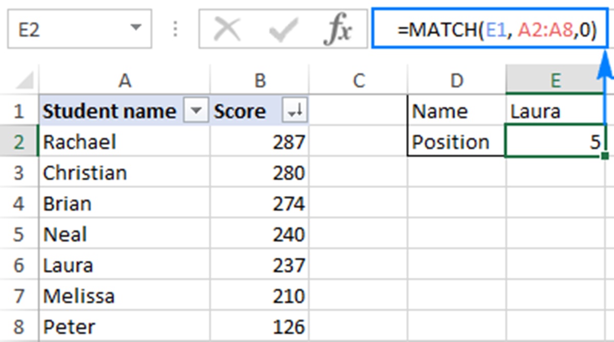
Example 3: Finding a value in a range of cells
The MATCH function in Excel is not limited to searching for values in a single column or row. It can also be used to find a value within a range of cells, which is particularly useful when working with a large dataset or when the data is not organized in a linear format.
Let’s consider the following example:
Suppose you have a spreadsheet that contains student names in column A and their corresponding scores in columns B, C, and D for different subjects. You want to find the score of a specific student in a specific subject. By using the MATCH function, you can easily locate the position of the student in column A and the position of the subject in the range of cells, and retrieve the corresponding score.
Here’s how you can achieve this:
Assuming the student names are listed in column A starting from cell A2, and the subjects are listed in row 1 starting from cell B1, you can use the following formula:
=INDEX(B2:D100, MATCH("John Doe", A2:A100, 0), MATCH("Math", B1:D1, 0))
In this example, the MATCH functions are used twice. The first MATCH function searches for the student name “John Doe” in column A and returns the position of the match. The second MATCH function searches for the subject “Math” in the range of cells B1:D1 and returns the position of the match. The INDEX function then retrieves the score from the corresponding location in the range B2:D100, based on the positions returned by the MATCH functions.
By utilizing the MATCH function with a range of cells, you can accurately and efficiently find and retrieve values within your dataset, regardless of how the data is organized.
Example 4: Using the MATCH function with other functions
The MATCH function in Excel can be combined with other functions to perform more advanced calculations or operations. By integrating the MATCH function with functions like SUM, AVERAGE, or COUNTIF, you can further analyze and manipulate your data.
Let’s explore an example:
Suppose you have a dataset that contains employee names in column A, their corresponding sales figures in column B, and the region they belong to in column C. You want to calculate the total sales for a specific region. By using the MATCH function together with the SUM function, you can easily accomplish this task.
Here’s an example:
Assuming the employee names are listed in column A starting from cell A2, their sales figures in column B, and the regions in column C, you can use the following formula:
=SUMIF(C2:C100, "Region A", INDEX(B2:B100, MATCH("Region A", C2:C100, 0)))
In this formula, the MATCH function is used to find the position of “Region A” within the range C2:C100. The INDEX function retrieves the corresponding sales figures from column B based on the position returned by the MATCH function. The SUM function then adds up all the sales figures that match “Region A” in column C.
By combining the MATCH function with other functions like SUM, AVERAGE, or COUNTIF, you can perform complex calculations and analysis on your data, providing valuable insights for your decision-making processes.
Example 5: Using the MATCH function with an approximate match
The MATCH function in Excel is not limited to exact matches. It can also be used with an approximate match to find the position of the closest value in a sorted range. This can be particularly useful when working with numerical data or when you need to perform range-based calculations.
Let’s consider the following example:
Suppose you have a dataset that contains a list of grades in column A, and you want to determine the grade category based on a given score. The grades are sorted in ascending order, and there are predefined score thresholds for each category.
Here’s an example:
| Grade | Score Threshold |
|---|---|
| Excellent | 90 |
| Good | 80 |
| Satisfactory | 70 |
| Needs Improvement | 60 |
To determine the grade category based on a given score, you can use the MATCH function with an approximate match, as shown in the following formula:
=INDEX(A2:A5, MATCH(B2, C2:C5, 1))
In this example, the MATCH function is used with a match_type of 1, indicating an approximate match. It searches for the value in cell B2 (the score) within the range C2:C5 (the score thresholds) and returns the position of the closest value that is less than or equal to the given score. The INDEX function then retrieves the corresponding grade category from the range A2:A5 based on the position returned by the MATCH function.
By using the MATCH function with an approximate match, you can dynamically assign grade categories based on specific score thresholds, allowing for flexible grading systems and efficient data analysis.
Tips and tricks for using the MATCH function effectively
The MATCH function is a powerful tool in Excel that can greatly enhance your data analysis and lookup operations. Here are some tips and tricks to help you make the most out of the MATCH function:
- Understand the match_type argument: The match_type argument in the MATCH function allows you to specify the type of match you want to perform. Make sure to choose the appropriate match_type (0, 1, or -1) based on your specific requirements.
- Use absolute cell references: When using the MATCH function in a formula, it’s recommended to use absolute cell references for the lookup_value and lookup_array to avoid any unexpected changes in the formula as you copy or move it to other cells in your worksheet.
- Combine with other functions: The MATCH function can be combined with other functions like INDEX, SUM, AVERAGE, or COUNTIF to perform more advanced calculations or lookup operations. Experiment with different combinations to achieve the desired outcome.
- Sort the range for approximate matches: For an approximate match with the MATCH function, ensure that the lookup_array is sorted in ascending or descending order, depending on the match_type. This will ensure accurate results and prevent any unexpected outcomes.
- Handle errors: If the MATCH function cannot find a match, it will return an error value (#N/A). You can use error handling functions like IFERROR or ISNA to handle these errors gracefully and provide alternative outputs or error messages.
- Practice with example datasets: To become comfortable and proficient with the MATCH function, practice using it with example datasets that simulate real-world scenarios. This will help you understand its capabilities and limitations.
By utilizing these tips and tricks, you can effectively harness the power of the MATCH function, allowing for efficient data analysis, improved lookup operations, and enhanced decision-making processes in Excel.