How to Use Excel's LOOKUP Function to Find Information

Overview of Excel’s LOOKUP Function

The LOOKUP function in Excel is a powerful tool that allows you to search for specific values in a range of cells and return information based on that search. Whether you want to find an exact match or an approximate match, the LOOKUP function provides a flexible way to extract data from your spreadsheet.

The syntax of the LOOKUP function is quite simple. You provide the search value and the lookup array, and Excel will find the matching value and return the corresponding value from the result array. The function can be used for both vertical and horizontal lookup, making it versatile for various data analysis tasks.

When it comes to finding an exact match, the LOOKUP function works by searching for the search value in the first column or row of the lookup array. Once a match is found, it retrieves the corresponding value from the result array. This makes it handy for tasks like looking up customer IDs or product codes to retrieve associated information.

If you need to find an approximate match, the LOOKUP function can still come to your rescue. It requires the lookup array to be sorted in ascending order. Excel will then locate the largest value in the lookup array that is less than or equal to the search value and return the corresponding value from the result array. This functionality is particularly useful when dealing with ranges such as finding the closest match to a given value in a set of data.

Understanding the lookup vector and the result vector is essential for effective use of the LOOKUP function. The lookup vector is the range of cells that Excel will search for the search value, while the result vector is the corresponding range from which the matching value will be retrieved. By specifying the correct vectors, you can ensure that Excel fetches the desired information from your spreadsheet.

One of the notable advantages of the LOOKUP function is its ability to handle errors gracefully. If the search value is not found in the lookup array, Excel returns the closest match if an approximate match was requested. Otherwise, it displays an error message, which can be customized to your liking. This feature helps prevent unexpected errors in your calculations and allows for efficient error handling within your spreadsheets.

While the LOOKUP function is a powerful tool on its own, it’s worth noting that there are alternative functions in Excel that can achieve similar results. The VLOOKUP and HLOOKUP functions, for instance, offer more specific versions of vertical and horizontal lookup respectively. The INDEX and MATCH functions provide additional flexibility for advanced lookup scenarios. Understanding the differences between these functions can help you choose the most appropriate one for your specific needs.

When using the LOOKUP function, there are a few tips and tricks that can enhance your productivity. For instance, using named ranges can make your formulas more readable and easier to maintain. You can also combine the LOOKUP function with other functions like IF or ISNA to handle specific conditions or errors. Exploring these techniques can help you harness the full potential of the LOOKUP function in Excel.

Syntax and Arguments of the LOOKUP Function

The LOOKUP function in Excel has a straightforward syntax and requires a few arguments to perform the desired search and retrieval of data. Understanding these arguments will enable you to utilize the function effectively in your spreadsheet tasks.

The basic syntax of the LOOKUP function is as follows:

=LOOKUP(lookup_value, lookup_vector, [result_vector])

The first argument, lookup_value, is the value that you want to find in the lookup_vector. This can be a cell reference, a text value, or a numerical value. You can even use a formula as the lookup_value, as long as it returns a valid value to search for.

The second argument, lookup_vector, is the range of cells where Excel will search for the lookup_value. This is often a single column or row, but it can also be a multiple column or row range.

The third argument, which is optional, is the result_vector. This argument specifies the range of cells from which Excel will extract the corresponding value if a match is found. If the result_vector is omitted, Excel will use the lookup_vector as the result_vector. However, if the result_vector is provided, it must have the same size or shape as the lookup_vector.

Excel also allows you to use additional optional arguments such as range_lookup and search_mode to further customize the behavior of the LOOKUP function. These arguments offer more advanced functionality, enabling you to control the exact search behavior and handling of error conditions. However, they are not commonly used unless you have specific requirements for your lookup tasks.

Using the correct syntax and understanding the available arguments of the LOOKUP function is crucial for accurate data retrieval in Excel. Make sure to provide the appropriate values for lookup_value, lookup_vector, and result_vector to ensure accurate search results. Additionally, being aware of the optional arguments can provide you with added control and flexibility when using the LOOKUP function.

Using LOOKUP to Find an Exact Match

The LOOKUP function in Excel is an excellent tool for finding an exact match in your spreadsheet data. By specifying the search value and the lookup array, you can easily retrieve the corresponding value from the result array.

To use the LOOKUP function for finding an exact match, follow these steps:

Ensure the lookup array is sorted in ascending order. The LOOKUP function requires the array to be sorted for accurate results.
Determine the search value, which can be a cell reference, a text value, or a numerical value. This value should match exactly with an entry in the lookup array.
Specify the lookup_vector as the range of cells where Excel will search for the search value. Typically, the lookup_vector is a single column or row but can also be a multiple column or row range.
If the result_vector is not provided, Excel will use the lookup_vector as the result_vector. However, if a specific result_vector is desired, provide it as the third argument.

By following these steps, the LOOKUP function will search for the search value within the lookup array. Once a match is found, Excel will return the corresponding value from the result_vector, providing you with the exact information you need.

It’s worth noting that the LOOKUP function searches for the search value in the first column or row of the lookup array. Therefore, make sure your search value corresponds to an entry in that specific column or row. If the search value is not found, the LOOKUP function will display an error, indicating that the value cannot be found in the lookup array.

Using the LOOKUP function for exact matches is particularly useful in scenarios where you have a unique identifier, such as a customer ID or product code, and want to retrieve specific information associated with that identifier. With just a few simple steps, you can harness the power of the LOOKUP function to quickly and accurately find the exact match you need in your Excel spreadsheets.

Using LOOKUP for Approximate Matches

The LOOKUP function in Excel is not limited to finding exact matches. It can also be used effectively for performing approximate matches, allowing you to find the closest value in a sorted range relative to your search value.

To use the LOOKUP function for approximate matches, follow these steps:

Ensure the lookup array is sorted in ascending order. The LOOKUP function requires the array to be sorted for accurate results.
Determine the search value, which can be a cell reference or a numerical value. This value should represent the point for which you want to find the closest match.
Specify the lookup_vector as the range of cells where Excel will search for the search value. Typically, the lookup_vector is a single column or row, but it can also be a multiple column or row range.
If the result_vector is not provided, Excel will use the lookup_vector as the result_vector. However, if a specific result_vector is desired, provide it as the third argument.

By following these steps, the LOOKUP function will locate the largest value in the lookup array that is less than or equal to the search value. It will then return the corresponding value from the result_vector, providing you with the closest match to your search value.

This functionality of the LOOKUP function is useful in various scenarios, such as finding the nearest value to a given number or determining the closest match in a set of data. It allows you to work with sorted ranges and identify values within those ranges that are closest to a target value.

It’s important to note that the lookup_vector must be sorted in ascending order for the LOOKUP function to work correctly when performing an approximate match. If the vector is not sorted, the function may return unexpected results. Additionally, if the search value falls outside the range of the lookup array, the LOOKUP function will return an error.

Using the LOOKUP function for approximate matches can greatly assist in tasks that require finding values that are close to a specific target. With its ability to search for the nearest value in a sorted range, the LOOKUP function provides flexibility and convenience in data analysis and decision-making processes within Excel.

Understanding the Lookup Vector and the Result Vector

The LOOKUP function in Excel relies on two key components: the lookup vector and the result vector. Understanding how these vectors work is essential for effectively using the LOOKUP function in your data analysis tasks.

The lookup vector is the range of cells in which Excel will search for the search value. This vector is typically a single column or row, but it can also be a multiple column or row range. When searching for a match, the LOOKUP function scans the first column or row of the lookup vector. It’s crucial to ensure that the search value corresponds to an entry in this specific column or row.

On the other hand, the result vector is the range of cells from which Excel will extract the corresponding value when a match is found. By default, if the result vector is not provided, Excel will use the lookup vector as the result vector. However, you have the option to specify a separate range for the result vector if needed.

It’s important to consider the size and shape of the lookup vector and the result vector to ensure accurate results. If the result vector is not the same size or shape as the lookup vector, Excel may return unexpected values or display errors.

Using the lookup vector and the result vector effectively allows you to extract specific information based on your search criteria. For example, if you have a column with product names and another column with corresponding prices, you can use the LOOKUP function to search for a specific product name in the lookup vector and retrieve the price from the result vector.

Understanding the relationship between the lookup vector and the result vector is crucial for accurate data retrieval. By specifying the correct vectors, you can ensure that Excel fetches the desired information from your spreadsheet, saving time and effort in your data analysis tasks.

When using the LOOKUP function with multiple columns or rows, ensure that the lookup vector and the result vector have the same size and shape for correct results. Additionally, always double-check that the search value corresponds to an entry in the first column or row of the lookup vector to obtain accurate and meaningful information.

Using LOOKUP with Multiple Columns or Rows

The LOOKUP function in Excel is not limited to searching for values in a single column or row. It can be used effectively with multiple columns or rows, allowing you to extract information based on complex search criteria.

When using the LOOKUP function with multiple columns or rows, you need to ensure that the lookup_vector and the result_vector have the same size and shape. This means that the number of columns and rows in both vectors should be identical.

Here’s how you can use the LOOKUP function with multiple columns or rows:

Create a lookup_vector and a result_vector with the same size and shape. These vectors can be ranges of cells, such as multiple columns or rows, that contain the data you want to search and retrieve information from.
Specify the lookup_vector as the range of cells where Excel will search for the search value. This vector can be a combination of columns or rows that you want Excel to scan for a match.
If the result_vector is not provided, Excel will use the lookup_vector as the result_vector. However, if you have a specific range from which you want to extract the corresponding value, provide it as the third argument.

Using the LOOKUP function with multiple columns or rows allows you to perform more complex searches and get specific information based on your criteria. For example, if you have a dataset with multiple columns representing different categories and you want to find the value associated with a particular combination of criteria, you can use the LOOKUP function with multiple columns to perform the search and extract the desired information.

It’s important to note that when using the LOOKUP function with multiple columns or rows, the first column or row of the lookup_vector will be searched for a match. Therefore, ensure that your search value corresponds to an entry in this specific column or row to obtain accurate results.

By leveraging the power of the LOOKUP function with multiple columns or rows, you can enhance your data analysis capabilities and retrieve specific information based on complex search criteria. This feature provides flexibility and versatility, enabling you to handle diverse data scenarios within Excel.

Handling Errors with the LOOKUP Function

The LOOKUP function in Excel includes error handling capabilities to help you deal with situations where the search value is not found or other unexpected errors occur. Understanding how to handle errors with the LOOKUP function is essential for ensuring accurate data retrieval in your spreadsheet.

When the LOOKUP function cannot find an exact match for the search value in the lookup_vector, it handles the situation differently depending on whether it is performing an exact match or an approximate match.

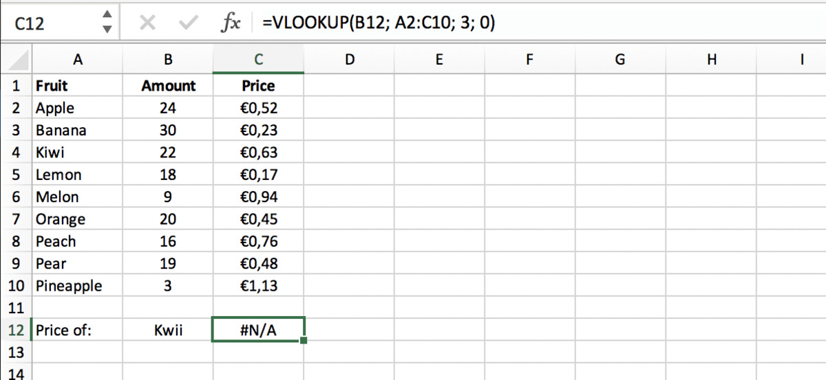
For exact matches, when the search value is not found in the lookup_vector, the LOOKUP function returns an error. This error message signifies that the value could not be found and can be customized to your preference. You can use different error-handling techniques in Excel, such as using the IF function or the ISNA function, to display a specific message or perform an alternative action when this error occurs.

When the LOOKUP function is used for approximate matches, it behaves differently. If the search value falls outside the range of the lookup array, the LOOKUP function returns an error. However, if the search value is within the range but does not match any exact values, Excel will return the nearest value in the lookup_vector that is less than or equal to the search value. This allows you to find approximate matches even when an exact match is not available.

Handling errors with the LOOKUP function is crucial for preventing unexpected results or inaccurate data retrieval. By customizing the error messages or applying alternative actions, you can ensure that your spreadsheets remain error-free and provide meaningful information.

Furthermore, when using the LOOKUP function in complex formulas or calculations, it’s essential to handle any potential errors that might arise. By incorporating error handling techniques, such as using the IF or ISNA functions, you can anticipate and handle errors in the LOOKUP function to ensure the reliability and accuracy of your calculations.

By effectively handling errors with the LOOKUP function, you can control how Excel responds to situations where the search value is not found or other unforeseen errors occur. This error handling capability enhances the robustness and accuracy of your spreadsheets, allowing for efficient data handling and analysis in Excel.

Comparing LOOKUP with Other Functions in Excel

While the LOOKUP function is a powerful tool for searching and retrieving information in Excel, it’s important to be aware of other functions that can achieve similar results. By comparing the LOOKUP function with other Excel functions, you can choose the most appropriate one for your specific needs.

Here are some key functions that are commonly compared to the LOOKUP function:

VLOOKUP: The VLOOKUP function is specifically designed for vertical lookups. It searches for a value in the leftmost column of a range and retrieves a corresponding value from another column. Compared to the LOOKUP function, VLOOKUP offers more specific functionality for vertical lookup scenarios.

HLOOKUP: The HLOOKUP function is similar to VLOOKUP but performs a horizontal lookup instead. It searches for a value in the top row of a range and retrieves a corresponding value from another row. HLOOKUP is useful when you have data organized horizontally instead of vertically.

INDEX and MATCH: The INDEX and MATCH functions are frequently used together as an alternative to the LOOKUP function. The INDEX function returns a value based on its position in an array, and the MATCH function searches for a specified value within an array and returns its position. By using INDEX and MATCH together, you can achieve more flexibility and control in your lookup operations.

When deciding which function to use, consider the specific requirements of your data analysis task. If you need a simple lookup function with basic functionality, the LOOKUP function may suffice. However, if you require more precise vertical or horizontal lookup capabilities, VLOOKUP or HLOOKUP may be more suitable.

Similarly, if you need to perform advanced lookups or search for values in arrays with complex structures, combining the INDEX and MATCH functions can provide greater versatility and accuracy.

It’s worth noting that each of these functions has its own syntax and unique functionality. Understanding the differences between them is crucial for choosing the right function for your specific needs. Consider factors such as the data orientation, required precision, and complexity of the lookup task to make an informed decision.

By comparing the LOOKUP function with other Excel functions and understanding their capabilities, you can leverage the most appropriate function to efficiently search, retrieve, and analyze data in your spreadsheets.

Tips and Tricks for Using the LOOKUP Function

The LOOKUP function in Excel provides a range of powerful features that can greatly enhance your data analysis tasks. To make the most of this function and improve your productivity, here are some valuable tips and tricks:

1. Use Named Ranges: Instead of referencing cell ranges directly in your LOOKUP function, consider using named ranges. Named ranges make your formulas more readable and easier to maintain, especially when working with large datasets or complex formulas.

2. Combine with IF Function: You can use the IF function in conjunction with the LOOKUP function to handle specific conditions or errors. For example, if the LOOKUP function returns an error, you can use the IF function to display a custom message or perform an alternative action.

3. Utilize Wildcards: When using the LOOKUP function for text-based searches, you can leverage wildcards such as asterisks (*) and question marks (?) to represent multiple or single characters. This allows for more flexible and expansive search criteria.

4. Sort Data before Performing Approximate Matches: To ensure accurate results when performing approximate matches, make sure to sort your lookup array in ascending order. This is crucial for Excel to locate the nearest value within the sorted array.

5. Combine with ISNA Function: The ISNA function can be used to check if the LOOKUP function returns an error value, such as when an exact match is not found. By using the ISNA function, you can handle these error conditions and provide specific actions or messages accordingly.

6. Experiment with Different Data Structures: The LOOKUP function can be used with various data structures, such as single columns, single rows, or multiple columns/rows. Take the time to experiment with different setups to find the most efficient and effective way to structure your data for Lookup operations.

7. Understand Search Order: The LOOKUP function searches for values based on the first column or row in the lookup array. Ensure that your search value corresponds to an entry in this specific column or row to obtain accurate and expected results.

8. Check for Data Integrity: Before using the LOOKUP function, double-check the data integrity in your lookup array. Ensure that there are no duplicate values or missing entries, as this can impact the accuracy of your lookup results.

By applying these tips and tricks, you can optimize your usage of the LOOKUP function and streamline your data analysis processes in Excel. These techniques will help you extract precise information, handle errors effectively, and improve overall efficiency in your spreadsheet tasks.