
What is an Array in Excel?
In Excel, an array is a collection or range of values that can be treated as a single entity. It allows you to perform calculations and operations on multiple values simultaneously, making complex calculations more efficient and easier to handle. Arrays in Excel can be one-dimensional (a single row or column of values) or two-dimensional (a matrix of values with rows and columns).
Arrays in Excel are incredibly powerful as they allow you to perform calculations on a large set of data with a single formula. This saves time and reduces the need for repetitive calculations. Array formulas also enable you to perform calculations that would be difficult or impossible with standard formulas, such as finding the maximum or minimum value in a range, counting unique values, or performing multi-criteria calculations.
To create an array formula in Excel, you need to use a special syntax. Instead of entering the formula in a single cell, you must enter it as an array formula over multiple cells. This is done by pressing Ctrl + Shift + Enter after entering the formula. Excel will automatically enclose the formula in curly braces { } to indicate that it is an array formula.
Arrays in Excel can be used with a wide range of functions and formulas, including mathematical operators, logical operators, text functions, lookup and reference functions, statistical functions, and even database functions. This versatility allows you to handle complex data analysis tasks and automate calculations efficiently.
However, it’s important to note that arrays in Excel have some limitations and considerations. First, array formulas can be resource-intensive and may slow down your Excel workbook if used extensively. Additionally, array formulas can be more challenging to understand and debug due to their complex nature. It’s crucial to carefully design and test your array formulas to ensure accurate results.
In the next sections, we will explore the advantages and limitations of using array formulas in Excel, as well as examples of how to use them with different functions and formulas. So, let’s dive deeper into the world of arrays and unleash the power of Excel’s array formulas!
How to Create an Array Formula in Excel
Creating an array formula in Excel allows you to perform calculations on multiple values simultaneously, making complex calculations more efficient. Here are the steps to create an array formula in Excel:
1. Select the range of cells where you want the array formula result to appear. Make sure the range has the same dimensions as the array you will be using in the formula.
2. Start entering the formula as you would with a regular formula, but instead of pressing Enter, press Ctrl + Shift + Enter. This tells Excel that you are entering an array formula.
3. Excel will automatically enclose the formula in curly braces { } to indicate that it is an array formula. Do not manually add these braces; Excel will add them automatically.
4. Once you have entered the formula and pressed Ctrl + Shift + Enter, the array formula will be applied to the selected range of cells, and the result will be displayed.
It’s important to note that when creating an array formula, you need to consider the relative references and absolute references carefully. Excel will adjust the references when the formula is applied to different cells in the array. To create absolute references, use the dollar sign ($) before the column letter or row number.
Here’s an example to illustrate how to create an array formula in Excel. Let’s say you have a range of numbers in cells A1 to A5, and you want to calculate the sum of the squares of these numbers.
1. Select the range of cells where you want the result to appear, let’s say B1 to B5.
2. Enter the formula “=A1:A5^2” (without quotes) in cell B1.
3. Instead of pressing Enter, press Ctrl + Shift + Enter.
4. Excel will enclose the formula in curly braces { }, and the result will be displayed in cells B1 to B5, showing the squared values of the numbers in cells A1 to A5.
Remember to always use Ctrl + Shift + Enter when creating an array formula to ensure it is applied correctly.
In the next sections, we will explore the advantages, limitations, and various applications of array formulas in Excel. So, let’s continue our journey to harness the power of array formulas!
Advantages of Using Array Formulas in Excel
Array formulas in Excel provide several advantages that can significantly enhance your spreadsheet calculations and data analysis. Here are the key advantages of using array formulas:
1. Efficient Calculation: Array formulas allow you to perform calculations on a large set of data with a single formula. This saves time and reduces the need for repetitive calculations. Instead of applying the formula to each individual data point, you can process the entire array in one go.
2. Simultaneous Operations: With array formulas, you can perform calculations on multiple values simultaneously. This is particularly useful when dealing with complex calculations that involve multiple criteria or conditions. You can combine functions and operators to perform advanced calculations in a single step.
3. Dynamic Range Selection: Array formulas can dynamically adapt to changes in the range of data. If you add or remove data points within the range, the formula automatically adjusts its calculations without the need for manual updates. This makes your spreadsheet more flexible and adaptable to changing data.
4. Advanced Data Analysis: Array formulas enable you to perform calculations that would be difficult or impossible with standard formulas. You can use array formulas to find the maximum or minimum value in a range, count unique values, or perform multi-criteria calculations. This opens up new possibilities for data analysis and decision-making.
5. Simplified Formulas: By using array formulas, you can simplify complex calculations into a single formula. This not only makes your formulas easier to manage and understand but also reduces the chances of errors. Instead of multiple nested formulas, you can create one clear and concise array formula.
6. Automation and Efficiency: With array formulas, you can automate repetitive calculations and streamline your workflow. By applying a single array formula to a range of cells, you can instantly calculate and update multiple results. This efficiency can greatly improve your productivity when working with large datasets.
Despite these advantages, it’s important to be mindful of the limitations and considerations of array formulas in Excel. Large arrays can slow down the performance of your workbook, and understanding and troubleshooting complex array formulas may require advanced formula knowledge.
In the next sections, we will explore the limitations of array formulas in Excel and delve into specific examples of how to use them with different functions and formulas. So, let’s continue our exploration of array formulas and uncover their practical applications in Excel!
Limitations and Considerations of Array Formulas in Excel
While array formulas in Excel offer great power and flexibility, it’s important to be aware of their limitations and considerations. Understanding these factors will help you make informed decisions when working with array formulas. Here are the key limitations and considerations of using array formulas in Excel:
1. Resource Intensive: Array formulas can be resource-intensive, especially when dealing with large arrays or complex calculations. Using extensive arrays or multiple complex array formulas can significantly slow down the performance of your Excel workbook. It’s important to carefully consider the size of your data and the computational requirements before applying array formulas.
2. Debugging Challenges: Array formulas can be more challenging to understand and debug compared to standard formulas. When encountering errors or unexpected results, it may take more time and effort to identify the cause and correct the issue. It’s crucial to test and validate your array formulas thoroughly to ensure accurate calculations.
3. Increased Complexity: Array formulas introduce an additional level of complexity to your spreadsheet. They may require the use of advanced formula techniques, such as nested functions and array-specific syntax. This complexity can make your workbook more difficult to maintain and update, particularly for users with limited formula knowledge.
4. Formula Length Limitation: Excel has a limitation on the maximum length of a formula, which can be a concern when working with complex array formulas. If your array formula exceeds this limit, you may need to break it down into smaller parts or explore alternative approaches to achieve the desired result.
5. Limited Compatibility: Array formulas are not always compatible with certain Excel features, such as some chart types, conditional formatting, or data validation rules. Before applying array formulas, it’s important to consider their impact on other aspects of your workbook and ensure compatibility with your desired functionality.
Despite these limitations, array formulas offer immense power and flexibility in performing complex calculations and data analysis. With proper planning, testing, and consideration of these limitations, you can harness the benefits of array formulas while mitigating potential challenges.
In the next sections, we will explore various examples of using array formulas with different functions and formulas in Excel. By understanding the practical applications of array formulas, you can leverage them effectively in your spreadsheet tasks. So, let’s dive into the world of array formulas and discover their versatility in Excel!
Array Functions in Excel
Excel provides a variety of built-in array functions that are specifically designed to work with arrays. These array functions enable you to perform complex calculations and manipulate arrays in a streamlined and efficient manner. Here are some commonly used array functions in Excel:
1. TRANSPOSE: This array function allows you to convert a vertical range of cells into a horizontal range, or vice versa. It transposes the rows and columns of an array to reorganize the data.
2. SUMPRODUCT: This function calculates the sum of the products of corresponding elements in multiple arrays. It is commonly used to perform calculations involving multiple criteria or conditions.
3. INDEX: This function returns the value of a cell in an array at a specified row and column number. It is useful for retrieving specific values from an array based on specified criteria.
4. SMALL and LARGE: These functions return the k-th smallest or largest values from an array. They are often used to find the minimum or maximum values in a range or to rank values within an array.
5. AVERAGEIF and AVERAGEIFS: These functions calculate the average of values in an array that meet specified criteria. AVERAGEIF is used for a single condition, while AVERAGEIFS is used for multiple conditions.
6. MAX and MIN: These functions return the maximum or minimum value from an array. They are commonly used to find the highest or lowest values in a range.
7. FREQUENCY: This function calculates the frequency distribution of values in an array. It calculates the number of values that fall within specified ranges or bins.
These are just a few examples of the array functions available in Excel. Each function has its own specific syntax and usage, and they can be combined with other functions and formulas to perform more advanced calculations.
To use an array function, you need to enter it as an array formula by pressing Ctrl + Shift + Enter. Excel will automatically apply the function to the entire array, producing a single result or an array of results.
Array functions are a powerful tool for data analysis and manipulation in Excel. By leveraging the capabilities of these functions, you can perform sophisticated calculations and gain valuable insights from your data.
In the following sections, we will explore how to use array formulas with logical operators, mathematical operators, text functions, lookup and reference functions, statistical functions, and even database functions in Excel. So, let’s continue our exploration of array formulas and unlock new possibilities for data analysis!
Using Array Formulas with Logical Operators in Excel
Logical operators allow you to perform comparisons and make logical decisions based on certain conditions in Excel. When combined with array formulas, they can help you perform complex calculations and filter data efficiently. Here’s how you can use array formulas with logical operators in Excel:
1. AND Function: The AND function is used to check if multiple conditions are TRUE. When used with array formulas, you can apply it to an array of values and determine if all the conditions are met in each corresponding element of the array.
Example: {=AND(A1:A5>0)} – This array formula checks if each value in the range A1:A5 is greater than 0 and returns TRUE or FALSE for each element.
2. OR Function: The OR function is used to check if at least one condition is TRUE. When used with array formulas, you can apply it to an array of values and determine if any of the conditions are met in each corresponding element of the array.
Example: {=OR(A1:A5>10)} – This array formula checks if any value in the range A1:A5 is greater than 10 and returns TRUE or FALSE for each element.
3. IF Function: The IF function allows you to perform conditional calculations based on a specified condition. When used with array formulas, you can apply it to an array of values and perform different calculations or return different values for each element based on the condition.
Example: {=IF(A1:A5>5, “Pass”, “Fail”)} – This array formula checks if each value in the range A1:A5 is greater than 5. If TRUE, it returns “Pass”, and if FALSE, it returns “Fail” for each element.
4. NOT Function: The NOT function is used to reverse the logical value of a condition. When used with array formulas, you can apply it to an array of values and determine if the condition is NOT TRUE in each corresponding element of the array.
Example: {=NOT(A1:A5=”Red”)} – This array formula checks if each value in the range A1:A5 is NOT equal to “Red” and returns TRUE or FALSE for each element.
By combining logical operators with array formulas, you can perform complex calculations, filter data based on multiple conditions, and make logical decisions on a large scale. This significantly enhances your ability to analyze data and make informed decisions in Excel.
In the following sections, we will explore how to use array formulas with mathematical operators, text functions, lookup and reference functions, statistical functions, and even database functions in Excel. So, let’s continue our exploration of array formulas and uncover their versatility in different scenarios!
Using Array Formulas with Mathematical Operators in Excel
Mathematical operators in Excel allow you to perform calculations and manipulate numerical data. When combined with array formulas, they enable you to perform mathematical operations on arrays of values efficiently. Here’s how you can use array formulas with mathematical operators in Excel:
1. Addition: The addition operator (+) is used to add values together. When used with array formulas, you can apply it to arrays of values and perform element-wise addition.
Example: {=A1:A5 + B1:B5} – This array formula adds the corresponding elements in the ranges A1:A5 and B1:B5.
2. Subtraction: The subtraction operator (-) is used to subtract values. When used with array formulas, you can apply it to arrays of values and perform element-wise subtraction.
Example: {=A1:A5 – B1:B5} – This array formula subtracts the corresponding elements in the ranges A1:A5 and B1:B5.
3. Multiplication: The multiplication operator (*) is used to multiply values. When used with array formulas, you can apply it to arrays of values and perform element-wise multiplication.
Example: {=A1:A5 * B1:B5} – This array formula multiplies the corresponding elements in the ranges A1:A5 and B1:B5.
4. Division: The division operator (/) is used to divide values. When used with array formulas, you can apply it to arrays of values and perform element-wise division.
Example: {=A1:A5 / B1:B5} – This array formula divides the corresponding elements in the ranges A1:A5 by B1:B5.
5. Exponentiation: The exponentiation operator (^) is used to raise values to a power. When used with array formulas, you can apply it to arrays of values and perform element-wise exponentiation.
Example: {=A1:A5 ^ B1:B5} – This array formula raises the corresponding elements in the range A1:A5 to the power of the elements in B1:B5.
By using the appropriate mathematical operators, you can perform complex mathematical calculations on arrays of values simultaneously. This saves time and simplifies the process of working with large datasets in Excel.
In addition to these basic mathematical operators, Excel also provides a range of mathematical functions, such as SUM, AVERAGE, MAX, MIN, and more. These functions can be combined with array formulas to perform advanced mathematical calculations on arrays of values.
In the following sections, we will explore how to use array formulas with text functions, lookup and reference functions, statistical functions, and even database functions in Excel. So, let’s continue our exploration of array formulas and discover their versatility in different scenarios!
Using Array Formulas with Text Functions in Excel
Text functions in Excel allow you to manipulate and analyze text data. When combined with array formulas, they enable you to efficiently perform operations on arrays of text values. Here’s how you can use array formulas with text functions in Excel:
1. CONCATENATE Function: The CONCATENATE function combines multiple strings of text into a single string. When used with array formulas, you can apply it to arrays of text values and concatenate them into a new array.
Example: {=CONCATENATE(A1:A5, ” “, B1:B5)} – This array formula concatenates the corresponding elements in the ranges A1:A5 and B1:B5, with a space in between.
2. LEN Function: The LEN function returns the length of a text string. When used with array formulas, you can apply it to arrays of text values and get the length of each string in the array.
Example: {=LEN(A1:A5)} – This array formula returns the length of each text string in the range A1:A5.
3. LEFT and RIGHT Functions: The LEFT and RIGHT functions extract a specified number of characters from the left or right side of a text string. When used with array formulas, you can apply them to arrays of text values and extract substrings from each string in the array.
Example: {=LEFT(A1:A5, 3)} – This array formula extracts the first three characters from each text string in the range A1:A5.
4. UPPER and LOWER Functions: The UPPER and LOWER functions convert text to uppercase or lowercase letters. When used with array formulas, you can apply them to arrays of text values and convert each string in the array to uppercase or lowercase.
Example: {=UPPER(A1:A5)} – This array formula converts each text string in the range A1:A5 to uppercase.
5. FIND Function: The FIND function searches for a specific text string within another text string and returns its position. When used with array formulas, you can apply it to arrays of text values and find the position of a substring in each string in the array.
Example: {=FIND(“apple”, A1:A5)} – This array formula searches for the substring “apple” in each text string in the range A1:A5 and returns the position of the substring.
By using these text functions with array formulas, you can efficiently manipulate and analyze arrays of text values in Excel. This gives you the ability to perform complex text operations and extract valuable insights from textual data.
In the following sections, we will explore how to use array formulas with lookup and reference functions, statistical functions, database functions, and more in Excel. So, let’s continue our exploration of array formulas and uncover their versatility in different scenarios!
Using Array Formulas with Lookup and Reference Functions in Excel
Lookup and reference functions in Excel enable you to search for specific values within a range or retrieve data from different parts of a worksheet. When combined with array formulas, they offer powerful tools for working with arrays of data. Here’s how you can use array formulas with lookup and reference functions in Excel:
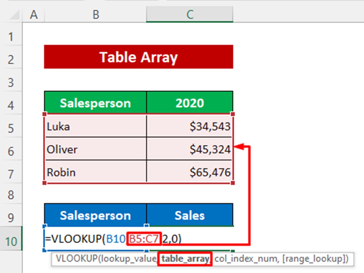
1. VLOOKUP Function: The VLOOKUP function searches for a specific value in the leftmost column of a range and returns a corresponding value from another column. When used with array formulas, you can apply it to arrays of values and retrieve multiple corresponding values.
Example: {=VLOOKUP(A1:A5, B1:D10, 2, FALSE)} – This array formula searches for each value in the range A1:A5 in the leftmost column of the range B1:D10 and returns the corresponding values from the second column.
2. HLOOKUP Function: The HLOOKUP function searches for a specific value in the top row of a range and returns a corresponding value from another row. When used with array formulas, you can apply it to arrays of values and retrieve multiple corresponding values.
Example: {=HLOOKUP(A1:A5, B1:D10, 3, FALSE)} – This array formula searches for each value in the range A1:A5 in the top row of the range B1:D10 and returns the corresponding values from the third row.
3. INDEX and MATCH Functions: The INDEX and MATCH functions work together to perform flexible lookups. When used with array formulas, you can apply them to arrays of values and retrieve multiple corresponding values based on specified criteria.
Example: {=INDEX(B1:D10, MATCH(A1:A5, C1:C10, 0), 2)} – This array formula searches for each value in the range A1:A5 in the range C1:C10 and returns the corresponding values from the second column of the range B1:D10.
4. INDIRECT Function: The INDIRECT function returns the value of a cell specified by a text string. When used with array formulas, you can apply it to arrays of text values and retrieve multiple values based on dynamically changing references.
Example: {=INDIRECT(A1:A5)} – This array formula converts the text references in the range A1:A5 into actual cell references and returns the corresponding values.
By using these lookup and reference functions with array formulas, you can efficiently search, retrieve, and dynamically reference data within arrays in Excel. They provide a powerful way to manage and analyze large datasets.
In the following sections, we will explore how to use array formulas with statistical functions, database functions, and more in Excel. So, let’s continue our exploration of array formulas and uncover their versatility in different scenarios!
Using Array Formulas with Statistical Functions in Excel
Statistical functions in Excel enable you to analyze and summarize data by calculating various statistical measures. When combined with array formulas, they allow you to perform statistical calculations on arrays of data efficiently. Here’s how you can use array formulas with statistical functions in Excel:
1. AVERAGE Function: The AVERAGE function calculates the arithmetic mean of a set of values. When used with array formulas, you can apply it to arrays of values and calculate the average for each corresponding element.
Example: {=AVERAGE(A1:A5)} – This array formula calculates the average of the values in the range A1:A5.
2. COUNT Function: The COUNT function counts the number of cells in a range that contain numeric values. When used with array formulas, you can apply it to arrays of values and count the number of values in each corresponding element.
Example: {=COUNT(A1:A5)} – This array formula counts the number of values in the range A1:A5.
3. MAX Function: The MAX function returns the maximum value in a range of values. When used with array formulas, you can apply it to arrays of values and find the maximum value for each corresponding element.
Example: {=MAX(A1:A5)} – This array formula returns the maximum value in the range A1:A5.
4. MIN Function: The MIN function returns the minimum value in a range of values. When used with array formulas, you can apply it to arrays of values and find the minimum value for each corresponding element.
Example: {=MIN(A1:A5)} – This array formula returns the minimum value in the range A1:A5.
5. SUM Function: The SUM function calculates the sum of a range of values. When used with array formulas, you can apply it to arrays of values and calculate the sum for each corresponding element.
Example: {=SUM(A1:A5)} – This array formula calculates the sum of the values in the range A1:A5.
These are just a few examples of statistical functions that can be used with array formulas in Excel. By applying these functions to arrays of values, you can perform statistical calculations and gain valuable insights into your data.
In the following sections, we will explore how to use array formulas with database functions, conditional functions, and more in Excel. So, let’s continue our exploration of array formulas and uncover their versatility in different scenarios!
Using Array Formulas with Database Functions in Excel
Database functions in Excel enable you to perform calculations and retrieve data from tables or databases. When combined with array formulas, they offer powerful tools for working with arrays of data in a structured manner. Here’s how you can use array formulas with database functions in Excel:
1. DSUM Function: The DSUM function calculates the sum of values in a database that meet specified criteria. When used with array formulas, you can apply it to arrays of database values and perform calculations on each corresponding element.
Example: {=DSUM(Database, “Sales”, Criteria)} – This array formula calculates the sum of “Sales” in the Database that meets the specified Criteria for each element.
2. DCOUNT Function: The DCOUNT function counts the number of records in a database that meet specified criteria. When used with array formulas, you can apply it to arrays of database values and perform counting operations on each corresponding element.
Example: {=DCOUNT(Database, “Region”, Criteria)} – This array formula counts the number of “Region” records in the Database that meet the specified Criteria for each element.
3. DAVERAGE Function: The DAVERAGE function calculates the average of values in a database that meet specified criteria. When used with array formulas, you can apply it to arrays of database values and perform averaging operations on each corresponding element.
Example: {=DAVERAGE(Database, “Revenue”, Criteria)} – This array formula calculates the average of “Revenue” in the Database that meets the specified Criteria for each element.
4. DMAX and DMIN Functions: The DMAX and DMIN functions return the maximum and minimum values in a database that meet specified criteria. When used with array formulas, you can apply them to arrays of database values and retrieve corresponding maximum and minimum values for each element.
Example: {=DMAX(Database, “Profit”, Criteria)} – This array formula returns the maximum “Profit” value in the Database that meets the specified Criteria for each element.
5. DGET Function: The DGET function retrieves a single value from a database that meets specified criteria. When used with array formulas, you can apply it to arrays of database values and retrieve corresponding values for each element.
Example: {=DGET(Database, “Product”, Criteria)} – This array formula retrieves the “Product” value from the Database that meets the specified Criteria for each element.
By using these database functions with array formulas, you can efficiently perform calculations, retrieve data, and analyze arrays of database values in Excel. They provide a systematic approach to working with structured data.
In the following sections, we will explore how to use array formulas with conditional functions, financial functions, and more in Excel. So, let’s continue our exploration of array formulas and uncover their versatility in different scenarios!
Examples of Using Array Formulas in Excel
Array formulas in Excel can be used in various scenarios to perform complex calculations, analyze data, and automate tasks. Here are a few examples showcasing the versatility of array formulas:
1. Summing a Range of Values:
Suppose you have a range of values in cells A1 to A5 and you want to calculate the sum of the squared values. You can use the following array formula:
{=SUM(A1:A5^2)}
This formula squares each value in the range A1:A5 and then calculates the sum of the squared values.
2. Finding Unique Values:
If you have a list of values in column A and you want to find the unique values, you can use the following array formula:
{=INDEX(A:A, MATCH(0, COUNTIF($B$1:B1, A:A), 0))}
This formula generates a list of unique values starting from cell B1 and expanding downwards. Each time the formula is entered, it finds the next unique value in column A and displays it in column B.
3. Running Totals:
To calculate a running total of a series of values, you can use the following array formula:
{=SUM($A$1:A1)}
This formula adds up the values in the range A1 to the current row and displays the running total. When entered, it calculates the running total for each row as it is dragged down.
4. Counting Occurrences:
Suppose you have a range of values in column A and you want to count how many times a specific value occurs in the column. You can use the following array formula:
{=SUM(IF(A1:A10=”Apple”, 1, 0))}
This formula counts the number of occurrences of the word “Apple” in the range A1:A10.
5. Multi-criteria Lookup:
If you have a dataset with multiple criteria and you want to retrieve a specific value based on those criteria, you can use the following array formula:
{=INDEX(D:D, MATCH(1, (A:A=”Category1″)*(B:B=”ProductX”), 0))}
This formula searches for the intersection of “Category1” in column A and “ProductX” in column B and returns the corresponding value in column D.
These examples illustrate the power and versatility of array formulas in Excel. By understanding and utilizing array formulas, you can streamline your calculations, automate tasks, and gain valuable insights from your data.
In the following sections, we will explore common errors and troubleshooting techniques related to array formulas, as well as the concept of table arrays in Excel. So, let’s continue our journey to master array formulas and enhance our Excel skills!
Common Errors and Troubleshooting with Array Formulas in Excel
Working with array formulas in Excel can sometimes be challenging, and errors are not uncommon. Understanding the common errors and troubleshooting techniques will help you identify and resolve issues more efficiently. Here are some common errors and troubleshooting tips related to array formulas:
1. Array Formula Syntax Error:
If you encounter a syntax error with an array formula, double-check the formula syntax, including the use of curly braces { } at the beginning and end of the formula. Remember to press Ctrl + Shift + Enter to enter the formula as an array formula.
2. Incorrect Results or Unexpected Output:
If your array formula is producing incorrect results or unexpected output, carefully review the formula logic and ensure that it is correctly applied to the desired range of cells. Double-check the range references and ensure they correspond correctly to the data you intend to use.
3. Array Range Mismatch:
When using array formulas, ensure that the arrays you are working with have matching dimensions. If the arrays have different sizes, it can lead to errors or incorrect results. Double-check the range sizes and make sure they align properly.
4. Performance Issues:
Working with large arrays or complex calculations can sometimes slow down your workbook’s performance. To improve performance, consider minimizing the number of array formulas used or restricting the range of cells to be calculated. You can also try using alternative formulas or techniques to achieve the desired result.
5. Array Calculation Mode:
By default, Excel uses automatic calculation mode, which can slow down the evaluation of array formulas. If you are working with a large array formula and experiencing performance issues, consider switching to manual calculation mode. You can do this by going to the Excel Options, selecting Formulas, and choosing Manual Calculation.
6. Evaluate Formula:
Excel provides an “Evaluate Formula” tool that allows you to step through the calculation process of a formula. This can help you identify any errors or issues within the array formula. Use the “Evaluate Formula” tool to troubleshoot problematic array formulas and understand how the calculations are being performed.
7. Debugging Techniques:
When troubleshooting array formulas, consider breaking down the formula into smaller parts to identify which component is causing the error. Use intermediate steps and examine the results at each stage to pinpoint the issue. You can use the F9 key to evaluate specific parts of the formula and isolate errors.
By being aware of these common errors and applying troubleshooting techniques, you can overcome challenges and ensure the correct functioning of your array formulas in Excel.
In the following sections, we will explore the concept of table arrays in Excel, how to create them, and the advantages they offer. So, let’s continue our exploration of Excel and enhance our skills with array formulas!
What is a Table Array in Excel?
In Excel, a table array is a structured range of data that is organized into rows and columns. It allows you to organize and manage data more efficiently, apply consistent formatting, and perform calculations and analysis more easily. A table array has several distinctive features that differentiate it from a regular range of cells in Excel.
Here are the key features and benefits of using a table array in Excel:
1. Structured Data Organization: A table array organizes your data into rows and columns, providing a clear structure. Each column represents a particular attribute or field, making it easier to understand and analyze your data.
2. Automatic Data Expansion: When adding new data to a table array, Excel automatically expands the table to accommodate the additional rows. This ensures that formulas, calculations, and formatting are applied consistently across the entire table.
3. Dynamic Named Ranges: Excel assigns a dynamic named range to each column in a table array. These named ranges adjust automatically as the table expands or contracts. You can use these named ranges in formulas and functions, simplifying your calculations and making them more flexible.
4. Sorting and Filtering: Table arrays allow you to sort and filter data easily. Excel applies a default filter to each column, enabling quick and convenient filtering of data based on specific criteria. Sorting the data by a particular column is equally effortless, allowing you to analyze and visualize your data more effectively.
5. Consistent Formatting: By applying a table style to a table array, Excel automatically formats the data and adds styling options such as alternating row colors and header formatting. This enhances the visual appeal of your data and makes it more readable.
6. Total Row Functionality: Table arrays have a built-in total row functionality that allows you to instantly calculate sums, averages, counts, and other statistical measures for selected columns. The total row adapts automatically as the table expands or contracts, ensuring accurate and up-to-date calculations.
7. Enhanced Data Analysis: Table arrays provide various tools for data analysis, such as the ability to create calculated columns, define structured references in formulas, and generate PivotTables and PivotCharts based on the table data. These features simplify data analysis and improve the accuracy of your calculations.
By using table arrays in Excel, you can efficiently organize and manage your data, automate calculations, and streamline your data analysis tasks. Table arrays provide a structured and dynamic way to work with your data, enhancing productivity and improving the reliability of your Excel workbooks.
In the following sections, we will explore how to create table arrays in Excel and dive deeper into the advantages they offer. So, let’s continue our journey of Excel proficiency and unleash the power of table arrays!
Creating a Table Array in Excel
Creating a table array in Excel is a straightforward process that allows you to efficiently organize and manage your data. Here are the steps to create a table array in Excel:
1. Select the data range: Highlight the range of cells containing your data, including the headers. Make sure all columns have unique headers, and there are no empty rows or columns within the range.
2. Convert to table: Go to the “Insert” tab on the Excel ribbon and click on the “Table” option. Excel will automatically detect the range, and a dialog box will appear showing the selected range for your table. Confirm that the range is correct and check the box indicating if your table has headers.
3. Style your table: Excel offers a variety of pre-defined table styles to choose from. Once your table is created, you can quickly select a style on the “Table Tools” tab, under the “Design” tab. Select a style to apply it to your table.
4. Customize your table: After creating the table, you can modify it to suit your needs. For example, you can resize columns, add or remove rows, insert calculated columns, rename columns, or format the table as desired.
5. Add a total row (optional): To enable the total row functionality, go to the “Table Tools” tab, and check the “Total Row” box under the “Table Style Options” group. Excel will automatically add a new row at the bottom of the table, which can be used to calculate totals or perform other summary calculations.
By following these steps, you can create a table array in Excel and take advantage of the benefits it offers. The table array provides a structured format for your data, automatic expansion, dynamic named ranges, sorting and filtering capabilities, consistent formatting, and enhanced data analysis tools.
Using table arrays in Excel improves the organization, manageability, and visualization of your data. It simplifies data manipulation, calculations, and analysis, making your Excel workbooks more efficient and reliable.
In the following sections, we will explore the advantages of using table arrays in Excel and how to leverage their features for data analysis and reporting. So, let’s continue our exploration of Excel and unlock the full potential of table arrays!
Advantages of Using Table Arrays in Excel
Table arrays in Excel provide numerous advantages that make data management, analysis, and reporting more efficient and user-friendly. Here are the key advantages of using table arrays in Excel:
1. Structured Data Organization: Table arrays allow you to organize your data into structured rows and columns, making it easier to navigate and understand. With clear headers, each column represents a specific attribute, enhancing data integrity and facilitating data analysis.
2. Automatic Data Expansion: When new data is added to a table array, Excel automatically expands the table to accommodate the new rows, ensuring that formulas, formatting, and data integrity are preserved. This eliminates the need for manual adjustments and ensures consistent calculations and formatting throughout the table.
3. Dynamic Named Ranges: Each column in a table array is automatically assigned a dynamic named range by Excel. These named ranges adjust automatically as the table expands or contracts, allowing for easy referencing in formulas and functions. The dynamic named ranges enhance formula readability and flexibility, simplifying calculations.
4. Sorting and Filtering: Table arrays offer built-in sorting and filtering options that can be easily accessed. With a few clicks, you can quickly sort your data by specific columns or filter data based on various criteria. This allows you to focus on specific subsets of data and perform detailed analysis effortlessly.
5. Consistent Formatting: By applying a table style to a table array, Excel automatically applies consistent formatting to the entire table. This includes alternating row colors, formatted headers, and standardized fonts and borders. Consistent formatting improves clarity and readability, enhancing the visual appeal of your data.
6. Total Row Functionality: Table arrays include a total row that provides convenient access to commonly used calculations, such as sum, average, count, and more. The total row adapts automatically as the table expands or contracts, ensuring accurate and up-to-date calculations. This eliminates the need to manually update formulas as data changes.
7. Simplified Data Analysis: Table arrays simplify data analysis by providing built-in features such as calculated columns, structured references, PivotTables, and PivotCharts. These features allow for quick and easy data summarization, aggregation, and visualization, enabling you to gain valuable insights and present data in a clear and concise manner.
Using table arrays in Excel enhances the efficiency and productivity of working with data. The structured organization, automatic data expansion, dynamic named ranges, sorting and filtering capabilities, consistent formatting, and simplified data analysis contribute to more effective data management and analysis.
In the following sections, we will explore how to leverage the features of table arrays for data analysis, reporting, and collaboration. So, let’s continue our exploration of Excel and unlock the full potential of table arrays!
Using Table Arrays with Formulas and Functions in Excel
Table arrays in Excel provide a powerful platform for utilizing formulas and functions to analyze and manipulate data effectively. The structured layout and dynamic features of table arrays make it easier to integrate formulas and functions into your data analysis workflow. Here’s how you can leverage table arrays with formulas and functions in Excel:
1. Structured References: Table arrays use structured references, which are an intuitive way to refer to specific columns in the table. Instead of using cell references, you can use the column headers as references in your formulas. This improves formula readability and makes them more resistant to errors when adding or deleting data in the table.
Example: Instead of using =SUM(A2:A10), you can use =SUM(Table1[Sales]) to calculate the sum of the “Sales” column in the table array named “Table1”.
2. Calculated Columns: Table arrays allow you to create calculated columns, which are columns that derive their values from formulas using data from other columns in the table. Calculated columns update automatically when the underlying data changes, providing real-time calculations and data analysis.
Example: You can create a calculated column in a table array that calculates the profit margin by dividing the “Profit” column by the “Revenue” column for each row in the table.
3. Total Row: The total row in a table array enables you to perform calculations on selected columns without the need for complex formulas. Simply choose the calculation you want to perform, such as sum, average, or count, from the drop-down menu in the total row, and Excel will automatically calculate the value based on the data in the corresponding column.
4. Array Functions: Array functions can also be used with table arrays to perform calculations on multiple values in a column or range within the table. These functions, such as AVERAGE, SUM, MAX, and MIN, operate on the entire column or range based on the data in the table array.
Example: =AVERAGE(Table1[Sales]) calculates the average of all the values in the “Sales” column of the table array named “Table1”.
By utilizing structured references, calculated columns, the total row, and array functions with table arrays, you can streamline your data analysis and reporting tasks in Excel. The built-in functionality of table arrays simplifies the utilization of formulas and functions, making data analysis more efficient and reducing the chances of errors.
In the following sections, we will explore how to use table arrays for advanced data analysis, reporting, and collaborating with others in Excel. So, let’s continue our journey of Excel proficiency and master the art of using table arrays!
Using Table Arrays with Data Analysis Tools in Excel
Table arrays in Excel seamlessly integrate with various data analysis tools, empowering you to gain valuable insights from your data. These tools leverage the structured layout and dynamic features of table arrays to facilitate advanced data analysis. Here’s how you can utilize table arrays with data analysis tools in Excel:
1. PivotTables: Table arrays are ideal for creating PivotTables, which enable you to summarize, analyze, and visualize data. PivotTables automatically recognize table array structures, making it easy to select the table as the data source. You can leverage the column headers as fields in the PivotTable, making the data analysis process more intuitive.
2. PivotCharts: When utilizing table arrays in combination with PivotTables, you can create dynamic and interactive PivotCharts. PivotCharts allow you to visualize your data in various chart types, such as column charts, line charts, or pie charts. Updating the PivotTable automatically updates the associated PivotChart, providing real-time data visualization.
3. Data Validation: Table arrays can be used in conjunction with data validation to create dropdown lists based on table column values. By referencing a table column as the source for the dropdown list, you ensure that the options in the list automatically update as new data is added to or removed from the table array.
4. What-If Analysis: The table array’s structured layout is beneficial when performing what-if analysis using tools like Data Tables or Goal Seek. These tools allow you to explore different scenarios and observe the impact on calculation results. You can easily reference table array columns in these tools to perform calculations and analyze the outcomes.
5. Statistical Formulas: Table arrays facilitate the application of statistical formulas and functions to the data. With structured references, you can use statistical functions such as AVERAGE, STDEV, or COUNTIFS directly on table array columns. These formulas automatically update as data changes, providing accurate and up-to-date statistical calculations.
6. Advanced Filter: Excel’s Advanced Filter feature seamlessly integrates with table arrays. You can specify criteria using table column headers and apply advanced filtering operations to extract specific data from the table. The structured layout of the table array simplifies the process of defining complex filtering criteria.
By leveraging table arrays with these data analysis tools in Excel, you can explore and manipulate data, uncover trends and patterns, and present insights to stakeholders more effectively. The structured format of table arrays enhances the functionality and usability of these tools, making the data analysis process more efficient and user-friendly.
In the following sections, we will explore practical examples of using table arrays for data analysis, reporting, and collaboration in Excel. So, let’s continue our exploration of Excel and unleash the full potential of table arrays!
Examples of Using Table Arrays in Excel
Table arrays in Excel offer a wide range of possibilities for data management, analysis, and reporting. Here are some examples showcasing the practical application of table arrays:
1. PivotTables and PivotCharts: Create a PivotTable using a table array to summarize and analyze sales data. Use the table’s columns as fields to group and analyze data by different dimensions, such as product, region, or year. Create a PivotChart based on the PivotTable to visualize the sales trends and patterns.
2. What-If Analysis: Utilize the table array in conjunction with Data Tables to perform what-if analysis. Explore different scenarios by changing input values and observe the impact on the calculated results. Data Tables automatically update the calculations based on the varying scenarios, allowing you to evaluate different outcomes.
3. Dynamic Charts: Build dynamic charts using table arrays to create visualizations that automatically update as new data is added. Use formulas that refer to the table array to define the chart ranges. Whenever new data points are added to the table array, the chart expands dynamically, ensuring the visualization remains up-to-date.
4. Advanced Filtering: Apply advanced filtering to a table array to extract specific data based on complex criteria. Use the structured layout of the table array to easily define filter conditions using column headers. This enables you to quickly extract relevant data from the table based on various criteria.
5. Statistical Analysis: Leverage the statistical functions and formulas available in Excel, such as AVERAGE, COUNTIFS, or STDEV, and apply them to the columns of a table array. Calculate summary statistics, filter data based on specific conditions, or perform more advanced statistical analysis on the table array data.
6. Data Validation: Use a table array as the source for data validation dropdown lists. Create dynamic dropdown lists that automatically update as new values are added or removed from the table array. This ensures that data validation dropdowns always reflect the most up-to-date data in the table.
These examples illustrate the versatility of table arrays in Excel, showcasing how they can be used to manage, analyze, and report on data. By harnessing the structured layout, automatic expansion, dynamic named ranges, and other features of table arrays, you can streamline your data-related tasks and gain valuable insights from your data.
In the following sections, we will explore additional tips and best practices for working with table arrays, further enhancing your proficiency in Excel. So, let’s continue our journey of Excel mastery and unlock the full potential of table arrays!