
The Basics of Excel
Excel is a powerful spreadsheet application developed by Microsoft that allows users to organize, analyze, and manipulate data. It is widely used in various industries and professions, from finance and accounting to project management and data analysis.
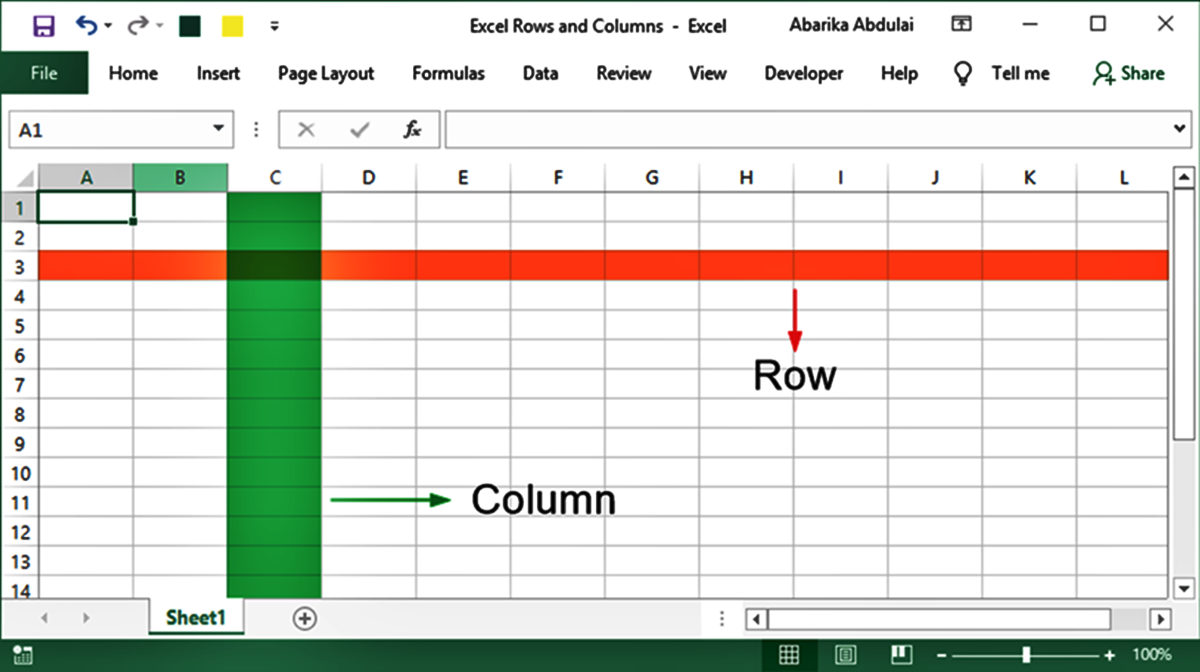
At its core, Excel is built on a grid system of cells, which are arranged in columns and rows. This grid-like structure forms the foundation of Excel’s functionality and serves as the backbone for organizing and storing data efficiently.
Each cell in Excel is identified by a unique coordinate, which consists of a column letter and a row number. For example, the cell at the intersection of column A and row 1 is referred to as cell A1. This naming convention makes it easy to reference and access specific cells within a spreadsheet.
Within the cells, you can input various types of data, such as numbers, text, dates, and formulas. Excel offers a wide range of functions and formulas that can perform complex calculations, automate tasks, and generate insights from the data.
One of the key features of Excel is its ability to create charts and graphs based on the data entered into the cells. These visual representations allow users to easily understand and communicate trends, patterns, and relationships within the data.
Furthermore, Excel provides powerful data manipulation tools, such as sorting and filtering, which allow users to organize and analyze large sets of data based on specific criteria. This functionality is particularly useful for data analysis, reporting, and decision-making purposes.
Excel also allows users to format cells, columns, and rows to enhance the visual appearance of the spreadsheet. This includes adjusting fonts and colors, applying borders and shading, and aligning text and numbers.
With its extensive range of features and versatility, Excel has become an indispensable tool for professionals who deal with data on a regular basis. Whether you are managing financial information, tracking project progress, or conducting data analysis, Excel provides the tools you need to make sense of your data and drive informed decisions.
Understanding Cells in Excel
In Excel, a cell is the basic building block of a spreadsheet. It is a rectangular box that can hold data such as numbers, text, dates, and formulas. Cells are arranged in a grid-like structure, with columns running vertically and rows running horizontally, forming a lattice of intersecting cells.
Each cell in Excel is identified by a unique coordinate, which consists of a column letter and a row number. For example, cell A1 is located in column A and row 1. This naming convention allows for easy reference and navigation within a spreadsheet.
Cells serve as the foundation for data entry and manipulation in Excel. You can enter different types of data into cells depending on your needs. Numeric data, such as sales figures or expenses, can be entered as numerical values. Text data, such as names or descriptions, can be entered as plain text. Dates and times can also be entered into cells, and Excel provides various date and time formatting options to display them in the desired format.
In addition to the above, cells can also contain formulas. Formulas are equations that perform calculations using the values in other cells. For example, you can use a formula to add up a column of numbers, calculate the average, or perform complex mathematical operations. Excel provides a wide range of built-in functions that can be used within formulas to perform various calculations and data manipulations.
One of the key advantages of using cells in Excel is their ability to be referenced and used in other cells. By referencing a cell in a formula, any changes made to the referenced cell will automatically update the result of the formula. This flexibility enables users to easily manipulate and analyze data within a spreadsheet.
Cells in Excel can also be formatted to enhance readability and presentation. This includes adjusting font styles and sizes, applying font colors and cell borders, and formatting numbers with specific decimal places or currency symbols. Formatting options are available for individual cells, as well as for entire columns or rows.
Understanding cells in Excel is essential for working effectively with spreadsheets. By utilizing the power of cells, you can input, manipulate, and analyze data, perform complex calculations, and create meaningful visualizations to make informed decisions.
What Are Columns in Excel?
In Excel, columns are the vertical sections of the spreadsheet that run from top to bottom. They are identified by letters of the alphabet, starting with column A and continuing to column Z. Once column Z is reached, the next column is labeled AA, AB, AC, and so on.
Columns in Excel provide a way to organize and categorize data by a specific attribute or type of information. For example, you can use a column to store names, dates, prices, quantities, or any other type of data that is relevant to your spreadsheet.
Each column has a default width, but you can adjust the width to accommodate the length of the data or to improve readability. This allows for a more organized and visually appealing spreadsheet.
Columns can also be utilized to perform calculations and data manipulations. By using formulas and functions, you can perform mathematical operations on the data in a column, such as adding, subtracting, multiplying, or averaging values. Excel provides a wide range of built-in functions that can be applied to columns to analyze and manipulate data.
Another advantage of using columns is the ability to sort and filter data. Excel allows you to sort a column of data in ascending or descending order based on its values. This makes it easy to arrange data in a desired order and identify trends or outliers.
Filtering data in a column allows you to selectively display data that meets specific criteria. You can filter a column by value, text, or condition to quickly narrow down the data and focus on what is relevant for your analysis or reporting.
Columns can also be used to create charts and graphs. By selecting a column or multiple columns, you can create visual representations of the data, such as bar charts, line graphs, or pie charts. These visualizations provide a clear and concise way to present data and highlight key insights.
What Are Rows in Excel?
In Excel, rows are the horizontal sections of the spreadsheet that run from left to right. They are identified by numbers, starting with row 1 and continuing in ascending order. Each row represents a unique record or entry in the spreadsheet.
Rows in Excel provide a way to organize and structure data in a logical order. Each row typically contains related information or data points that pertain to a specific record or category. For example, in a sales spreadsheet, each row may represent a different sale, with columns for the customer name, product sold, quantity, price, and total.
Similar to columns, rows have a default height, but you can adjust the height to accommodate the content within the cells. This allows for better visibility and readability of the data in the spreadsheet.
Rows can also be utilized for calculations and data analysis. By using formulas and functions, you can perform calculations across a row, such as summing up values, finding averages, or determining the maximum or minimum values. These calculations can provide valuable insights and help in making informed decisions based on the data.
Excel allows you to sort rows based on the values in a specific column. Sorting rows can be useful for arranging data in a specific order, such as sorting customer names alphabetically or sorting dates in chronological order. This feature can greatly facilitate data analysis and reporting.
Filtering rows allows you to display only specific records or data that meet certain criteria. You can apply filters to a particular column to show or hide rows based on value, text, or condition. Filtering rows provides a convenient way to focus on specific subsets of data and extract relevant information.
Rows are also crucial for data entry and data organization. When entering data into a spreadsheet, each record or data point is typically placed in a separate row. Rows help maintain the integrity and structure of the dataset, allowing for easy updates and modifications.
Additionally, rows play a significant role in data visualization. Excel allows you to create charts and graphs based on row data, enabling you to present trends, patterns, and comparisons visually. Whether it’s a bar graph, line graph, or scatter plot, using rows as the basis for data visualization can enhance understanding and communication.
How Columns and Rows Work Together
In Excel, columns and rows work together harmoniously to create a structured and organized grid-like system for managing and analyzing data. The intersection of a column and a row forms a cell, which holds specific data within the spreadsheet. Understanding how columns and rows interact is essential for effectively utilizing Excel’s functionality.
Columns and rows allow for the efficient organization of data within a spreadsheet. Columns provide a vertical structure, allowing you to categorize and classify data by different attributes or variables. On the other hand, rows provide a horizontal structure, representing individual records or entries in the spreadsheet. Together, they form a grid that ensures the data is arranged logically and can be easily referenced and manipulated.
By using columns and rows, you can create a comprehensive data table with each data point occupying its respective cell. This ensures that data remains organized and coherent, making it easier to perform calculations, analyze trends, and generate meaningful insights.
Columns and rows also work seamlessly with Excel’s powerful functions and formulas. By referencing specific cells in formulas, you can perform calculations that span across multiple columns and rows. This allows for advanced data analysis and enables you to derive meaningful results from the data in your spreadsheet.
Additionally, columns and rows play a vital role in data visualization. Excel’s charting capabilities allow you to create visual representations of your data, such as bar graphs, line charts, or pie charts. These visualizations are based on the data in the columns and rows, providing a clear and concise presentation to convey information effectively.
Furthermore, columns and rows offer flexibility when it comes to sorting and filtering data. You can sort data by one or more columns, rearranging the rows based on specific criteria. This allows you to identify patterns, rank values, and highlight important information. Filtering data allows you to selectively display rows that meet certain conditions or criteria, enabling you to focus on specific subsets of data for analysis or reporting purposes.
Overall, columns and rows work hand in hand to create a well-structured and organized environment for managing and analyzing data in Excel. By leveraging the power of columns and rows, you can input, manipulate, and visualize data efficiently, empowering you to make informed decisions and gain valuable insights from your data.
Selecting Columns and Rows in Excel
In Excel, selecting columns and rows is a fundamental step in working with data efficiently. It allows you to perform various tasks such as entering data, formatting cells, applying formulas, sorting, filtering, and more. Understanding how to select columns and rows effectively can greatly enhance your productivity and streamline your work in Excel.
To select an entire column, simply click on the column letter at the top of the spreadsheet. For example, to select column A, click on the letter “A”. The entire column will be highlighted to indicate it is selected. To select multiple columns, hold down the Ctrl key on your keyboard and click on the column letters you want to include in the selection.
Selecting an entire row follows a similar process. Click on the row number on the left side of the spreadsheet to select the entire row. For example, click on the number “1” to select row 1. To select multiple rows, hold down the Ctrl key and click on the row numbers you want to include in the selection.
If you want to select a specific range of cells that span multiple columns and rows, click and drag the mouse pointer over the desired range. This will create a highlighted area to indicate the selected range.
Excel also provides shortcuts for selecting columns and rows. To select an entire column, you can press Ctrl + Spacebar. This selects the entire column of the active cell. To select an entire row, you can press Shift + Spacebar. This selects the entire row of the active cell.
Another useful technique for selecting columns and rows is to use the “Select All” button. It is located in the top-left corner of the spreadsheet, where the column headers and row numbers intersect. Clicking on this button once will select the entire worksheet.
Once columns or rows are selected, you can perform various actions on them. For example, you can insert or delete columns or rows to modify the structure of the spreadsheet. You can also format the selected columns or rows by changing the font, applying cell borders, or adjusting the column width or row height.
In addition, selected columns or rows can be sorted or filtered to rearrange or refine the data. Excel provides options to sort in ascending or descending order based on the values in the selected columns. Filtering allows you to display specific subsets of the data based on criteria you define.
By mastering the art of selecting columns and rows in Excel, you can efficiently work with your data, manipulate the structure of your spreadsheet, and perform various operations to meet your specific needs.
Inserting and Deleting Columns and Rows
Excel provides the flexibility to insert and delete columns and rows as needed, allowing you to modify the structure and layout of your spreadsheet. This functionality is essential for organizing and managing your data effectively. Whether you need to add new columns for additional data or remove unnecessary rows, Excel makes it easy to make these adjustments.
To insert a column, simply select the column letter to the right of where you want the new column to be inserted. Right-click on the selected column and choose “Insert” from the context menu. Excel will insert a new column to the left of the selected column. Alternatively, you can use the “Insert” command from the toolbar or ribbon, which also allows you to choose the option to insert an entire column.
Inserting a row is a similar process. Select the row number below where you want the new row to be inserted. Right-click on the selected row and choose “Insert” from the context menu. Excel will insert a new row above the selected row. Additionally, you can use the “Insert” command from the toolbar or ribbon, and select the option to insert an entire row.
If you want to delete a column, select the column letter of the column you want to delete. Right-click on the selected column and choose “Delete” from the context menu. Excel will remove the selected column and adjust the rest of the columns accordingly. Similarly, you can use the “Delete” command from the toolbar or ribbon and choose the option to delete the entire column.
Deleting a row follows the same concept. Select the row number of the row you want to delete. Right-click on the selected row and choose “Delete” from the context menu. Excel will delete the selected row and shift the remaining rows up. The “Delete” command from the toolbar or ribbon can also be used to delete the entire row.
It’s important to note that when you insert or delete columns and rows, any data or formatting within the affected area will be shifted or adjusted accordingly. Make sure to review the changes to ensure the desired outcome.
In addition to manually inserting and deleting columns and rows, Excel also provides shortcuts for these actions. To insert a column, select the column, and press Ctrl + Shift + “+”. To insert a row, select the row and press Ctrl + Shift + “+”. To delete a column, select the column and press Ctrl + “-“. To delete a row, select the row and press Ctrl + “-“.
By mastering the skills of inserting and deleting columns and rows in Excel, you can effectively customize and manage the structure of your spreadsheet, allowing you to organize and manipulate your data in a way that best suits your needs.
Modifying Column and Row Widths
In Excel, modifying column and row widths is a crucial aspect of formatting and customizing your spreadsheet to ensure optimal visibility and readability of data. Adjusting the widths of columns and rows allows you to accommodate varying amounts of content, improving the overall appearance and usability of your spreadsheet.
To modify the width of a column, position your cursor on the vertical gridline to the right of the column letter in the column header. The cursor will change to a double-sided arrow. Click and drag the gridline to the right or left to increase or decrease the width of the column, respectively. Alternatively, you can select the column, go to the “Home” tab in the toolbar, and use the “Format” option to adjust the column width.
Similarly, to modify the height of a row, position your cursor on the horizontal gridline below the row number in the row header. The cursor will change to a double-sided arrow. Click and drag the gridline up or down to increase or decrease the height of the row, respectively. Alternatively, select the row, go to the “Home” tab in the toolbar, and use the “Format” option to adjust the row height.
If you want to modify the widths of multiple columns or heights of multiple rows simultaneously, select the desired columns or rows by clicking and dragging your mouse or by holding down the Ctrl key and clicking on the column letters or row numbers. After selecting the columns or rows, follow the same procedure mentioned above to adjust their respective widths or heights.
Excel also provides automatic column width adjustment based on the content within the cells. A quick way to adjust a column to fit its content is to double click on the right border of the column header. Excel will automatically resize the column width to accommodate the longest content within the cells of that column.
Additionally, Excel allows you to set specific column widths or row heights using numerical values. Select the desired columns or rows, go to the “Home” tab in the toolbar, and enter the preferred width or height values in the “Column Width” or “Row Height” options, respectively. This method ensures consistency across multiple columns or rows.
By modifying column and row widths in Excel, you can customize your spreadsheet to effectively display your data, improve readability, and create a well-structured document. Proportional and appropriate widths and heights of columns and rows enhance the visual presentation and make working with data more efficient.
Formatting Columns and Rows
In Excel, formatting columns and rows allows you to enhance the visual appearance and organization of your spreadsheet. By applying formatting options, you can emphasize important data, improve readability, and create a more professional and polished look for your document.
Excel offers a wide range of formatting options for columns and rows. Here are some common formatting techniques:
- Font formatting: You can change the font style, size, and color of the text within cells. This allows you to highlight specific data or make it more visually appealing.
- Cell borders: Adding borders to cells, columns, or rows can help separate and delineate different sections of your data. You can choose from various border styles and thicknesses.
- Cell shading: Applying shading or background colors to cells can create a more visually appealing and organized appearance. You can choose from a variety of colors to match your desired theme or highlight specific data.
- Number formatting: Excel provides the ability to format numbers in different ways, such as applying currency symbols, decimal places, or percentage formats. This allows for consistency and readability of numeric data.
- Alignment: Adjusting the alignment of data within cells can improve readability. You can align text to the left, right, or center within cells, as well as vertically align it at the top, middle, or bottom of the cell.
- Column/Row headers: You can format the headers of your columns and rows differently to distinguish them from the rest of your data. For example, you can apply bold formatting or a different font color to make them stand out.
To format columns and rows, select the desired columns or rows by clicking and dragging your mouse or by holding down the Ctrl key and clicking on the column letters or row numbers. Once selected, you can apply formatting options from the toolbar or ribbon. Alternatively, right-click on the selected columns or rows and choose the “Format Cells” option to access more advanced formatting settings.
Excel also allows you to quickly copy formatting from one column or row to another. Simply select the column or row that has the desired formatting, click on the “Format Painter” button in the toolbar, and then click on the target column or row that you want to apply the formatting to. The formatting will be copied over instantly.
By formatting columns and rows in Excel, you can enhance the visual appeal of your spreadsheet, make it easier to read and understand, and draw attention to key information. Consistent and well-organized formatting creates a professional and polished look, improving the overall presentation of your data.
Sorting Data by Columns or Rows
In Excel, sorting data by columns or rows is a powerful feature that allows you to rearrange your data in a specific order based on the values in a chosen column or row. Sorting data helps to identify trends, patterns, and outliers, making it easier to analyze and interpret your data effectively.
To sort data in Excel, start by selecting the range of cells that you want to sort. This could be a single column or an entire table that includes multiple columns and rows. Once you have selected the range, go to the “Data” tab in the toolbar and click on the “Sort” button.
In the “Sort” dialog box, you can choose the column or row by which you want to sort the data. Select the appropriate column or row from the “Sort by” or “Column” drop-down menu. You can also specify whether you want to sort the data in ascending order (from the lowest to the highest values) or descending order (from the highest to the lowest values).
Excel also allows you to sort data using multiple levels or criteria. This is useful when you want to sort data by one column and then by another column within the same dataset. To do this, click on the “Add Level” button in the “Sort” dialog box and specify the additional column and sorting order.
Once you have defined the sorting options, click on the “OK” button to apply the sorting to your selected range. Excel will rearrange the data based on the chosen column or columns, resulting in a new order of rows or columns.
Sorting data is particularly useful when you want to organize data alphabetically, numerically, or chronologically. For example, you can sort a column containing names in alphabetical order, a column with sales figures in ascending order, or a column with dates in chronological order. Sorting makes it effortless to identify the highest or lowest values in a dataset, identify duplicates, or locate specific information quickly.
It’s important to note that when sorting data, Excel will adjust the positions of the entire rows or columns, preserving the relationship between the cells within each row or column. This ensures that all the associated data stays intact and remains aligned.
By utilizing the sorting feature in Excel, you can easily organize and analyze your data to gain valuable insights. Sorting data enables you to identify trends, outliers, and patterns, making your data more manageable and meaningful.
Filtering Data by Columns or Rows
In Excel, filtering data by columns or rows is a powerful feature that allows you to selectively display specific subsets of data based on certain criteria. By applying filters to your data, you can easily analyze, sort, and extract relevant information from large datasets, saving time and improving productivity.
To filter data in Excel, start by clicking on any cell within your dataset. Then, go to the “Data” tab in the toolbar and click on the “Filter” button. Excel will automatically add filter dropdown arrows to the header row of each column in your dataset.
Once the filter dropdown arrows are visible, you can click on any of them to access a list of unique values within that column. By selecting or deselecting specific values, you can filter the dataset to display only the rows that meet the selected criteria. You can also utilize the search function within the filters to quickly find specific values within the column.
In addition to filtering by individual values, Excel provides various filter options and criteria to refine your data further. You can filter data based on text filters, number filters, date filters, or even custom filters where you can specify your own criteria using operators such as greater than, less than, equal to, and more.
Excel also allows for advanced filtering options, such as filtering by color, filtering by top or bottom values, or applying multiple filters across different columns.
Filtering data is particularly useful when working with large datasets or when you need to focus on specific subsets of data. For example, you may want to filter a sales dataset to display only the transactions from a specific region, or filter a customer database to show only the records of active customers.
Filtered data can be easily sorted within the filtered range based on any column or combination of columns. This allows you to further refine and analyze the data without affecting the original dataset. It’s important to note that filtered data does not alter or delete any rows from the original dataset. The filter simply hides the rows that do not meet the selected criteria, making it easy to revert back to the original dataset.
To remove the filters and display the entire dataset again, click on the filter dropdown arrows and select the “Clear Filter” option.
By utilizing the filtering feature in Excel, you can quickly and efficiently analyze and extract specific subsets of data that are relevant to your analysis or reporting needs. Filtering enables you to focus on the most important information and allows for deeper insights into your dataset.
Using Formulas and Functions with Columns and Rows
Excel’s true power lies in its ability to perform calculations and data manipulation using formulas and functions. By utilizing formulas and functions with columns and rows, you can automate complex calculations, analyze data, and derive valuable insights from your spreadsheet.
Formulas in Excel are expressions that perform calculations using the values in cells. They can include mathematical operators, cell references, and functions. Functions, on the other hand, are predefined formulas that perform specific operations or calculations.
To use formulas with columns and rows, you can reference specific cells within the formula. For example, you can add up the values in a column by using the SUM function and specifying the range of cells to be included in the calculation. This allows you to easily perform calculations on large sets of data without manually entering each individual value.
Excel provides a vast library of built-in functions that you can use with columns and rows. These functions range from basic arithmetic operations, such as SUM, AVERAGE, and MAX, to more advanced functions, such as VLOOKUP, IF, and COUNTIF. These functions enable you to perform complex calculations, analyze data based on specific conditions, and extract valuable information from your dataset.
When using formulas and functions with columns and rows, it’s important to understand how cell referencing works. Excel utilizes both relative and absolute cell references. A relative cell reference adjusts automatically when a formula is copied to other cells. An absolute cell reference, denoted by a dollar sign in the formula, remains constant when the formula is copied to other cells.
By utilizing formulas and functions, you can quickly perform calculations across multiple columns and rows. For example, you can calculate the total sales for a specific period by using the SUM function with a range of cells in a sales column. You can calculate the average monthly expenses by using the AVERAGE function with a range of cells in an expenses column.
Formulas and functions can also be combined and nested to perform more complex calculations. You can use logical functions, such as IF, to perform calculations based on certain conditions. You can use mathematical functions, such as ROUND, to round values to a specific decimal place. The possibilities are almost endless, allowing you to tailor your calculations to your specific needs.
By using formulas and functions with columns and rows in Excel, you can automate calculations, analyze data, and derive insights to make informed decisions. The ability to perform complex calculations and data manipulation unlocks the full potential of Excel as a powerful tool for data analysis and management.
Creating Charts Based on Columns and Rows
One of the key features of Excel is its ability to create charts and visual representations of data based on columns and rows. Charts provide a dynamic and visually appealing way to analyze and present information, making it easier to understand trends, patterns, and comparisons within your data.
To create a chart in Excel, start by selecting the range of cells that you want to include in the chart. This range can be a single column, multiple columns, or even a combination of columns and rows. Once the range is selected, go to the “Insert” tab in the toolbar and choose the type of chart you want to create from the available options.
Excel offers a variety of chart types, including column charts, bar charts, line charts, pie charts, and more. Each chart type is best suited for presenting different types of data and highlighting specific insights. For example, a column chart is ideal for comparing data across categories, while a line chart is suitable for showing trends over time.
Once you have selected a chart type, Excel will generate a chart based on the selected data range. The chart will be embedded in your worksheet, allowing you to resize and reposition it as needed. Additionally, Excel provides various customization options to modify the appearance and layout of your chart.
You can customize the chart by adding or removing chart elements such as titles, legends, and data labels. You can also adjust the formatting options for the axis labels, gridlines, and data markers. Excel’s formatting tools allow you to change colors, fonts, and other visual properties to match your desired style or branding.
Excel also allows you to create combination charts, which incorporate multiple chart types into a single chart. This is useful when you want to compare different types of data or present multiple metrics within a single visualization.
Once the chart is created, it is linked to the original data range. Any changes made to the data will automatically update the chart accordingly, ensuring that your chart always reflects the latest information.
Charts in Excel provide a powerful way to convey data visually, making it easier to understand and interpret complex information. They are particularly useful for presentations, reports, and data analysis. By creating charts based on columns and rows, you can effectively communicate insights, identify patterns, and make data-driven decisions.
Applying Conditional Formatting to Columns and Rows
Conditional formatting is a powerful feature in Excel that allows you to automatically apply formatting styles to cells, columns, or rows based on specific conditions or criteria. By using conditional formatting, you can highlight important data, identify trends, or draw attention to specific values within your spreadsheet.
To apply conditional formatting in Excel, select the range of cells, columns, or rows that you want to format. Then, go to the “Home” tab in the toolbar and click on the “Conditional Formatting” button. From the dropdown menu, you can choose from various pre-defined rules or create custom rules to apply the desired formatting.
Excel provides a wide range of built-in formatting options for conditional formatting. These include highlighting cells that meet certain criteria, such as greater than, less than, equal to, between, or containing specific values. You can apply different formatting, such as font color, fill color, or data bars, to the cells that meet the specified conditions.
Conditional formatting can be applied to individual cells within a column or row, making it easy to identify outliers or specific data points. It can also be applied to entire columns or rows, allowing you to visually distinguish specific trends or patterns across your data.
Excel also provides the ability to create complex conditional formatting rules by using formulas. This allows you to apply conditional formatting based on more advanced criteria or calculations. For example, you can highlight cells that contain a specific word or phrase, cells that fall within a certain date range, or cells that meet multiple conditions using logical operators.
Once the conditional formatting rules are applied, any changes to the underlying data that affect the conditions will automatically update the formatting accordingly. This dynamic feature ensures that the conditional formatting remains relevant and up-to-date, even as the data changes.
Conditional formatting can be a powerful tool for visualizing and analyzing your data. By applying conditional formatting to columns and rows, you can quickly identify key insights, spot trends, and draw attention to critical information within your spreadsheet.
Using conditional formatting effectively can significantly enhance the readability and impact of your data, making it easier to understand and interpret. Whether you are highlighting outliers, emphasizing trends, or highlighting specific values, conditional formatting helps you present your data visually and effectively.
Consolidating Data from Multiple Columns or Rows
Consolidating data from multiple columns or rows is a useful feature in Excel that allows you to combine and summarize information from different parts of your spreadsheet into a single location. It can be particularly helpful when you need to analyze or report on data that spans across multiple columns or rows.
To consolidate data in Excel, start by selecting the destination cell or range where you want the consolidated data to appear. This could be a new column, a new row, or even a separate sheet within the same workbook.
Next, go to the “Data” tab in the toolbar and click on the “Consolidate” button. In the “Consolidate” dialog box, you can specify the ranges of cells that you want to consolidate. You can select cells from different columns or rows by clicking on the “Add” button and choosing the appropriate range.
Excel provides several consolidation functions that you can choose from, based on how you want to summarize or consolidate the data. Some common consolidation functions include sum, average, count, min, max, and more. You can apply these functions to the consolidated data to calculate totals, averages, counts, or other summary values.
If your data is organized in a regular pattern, you can use the “Labels” option to consolidate data by category or label. This allows you to consolidate data that shares the same label or category. Excel will automatically group and summarize the data based on the labels.
Additionally, Excel provides options for handling duplicate data during the consolidation process. You can choose to include or exclude duplicate values, or you can decide how to handle them based on specific criteria.
Once you have specified the ranges and consolidation options, click on the “OK” button to consolidate the data. Excel will merge the selected data into the destination range according to your specified consolidation function or method.
Consolidating data is useful for creating summary reports or analyzing data across different columns or rows. It allows you to quickly retrieve important information and gain insights from multiple sources of data.
By consolidating data from multiple columns or rows, you can bring together related information, identify patterns or trends, and generate a consolidated view of your data. This consolidation process facilitates analysis, reporting, and decision-making based on the combined information.
Tips and Tricks for Working with Columns and Rows in Excel
Working with columns and rows in Excel can be made easier and more efficient with the help of some tips and tricks. These techniques can enhance your productivity and help you effectively organize, manipulate, and analyze data. Here are some useful tips to optimize your workflow:
- Freezing columns or rows: To keep certain columns or rows visible while scrolling through a large dataset, you can freeze them. Select the column or row that you want to freeze, go to the “View” tab in the toolbar, and click on “Freeze Panes.”
- Changing column width/row height quickly: To automatically adjust the width of a column or the height of a row to fit the content, double-click on the right boundary of the column header or the bottom boundary of the row header.
- Copying column/row formatting: To quickly copy the formatting of a column or row to another, select the source column or row, click on the “Format Painter” button in the toolbar, and then click on the destination column or row.
- Selecting entire columns or rows: To quickly select an entire column, click on the column letter at the top of the spreadsheet. To select an entire row, click on the row number on the left side of the spreadsheet. Alternatively, use the shortcut Ctrl + Spacebar to select a column and Shift + Spacebar to select a row.
- Applying filters: To quickly apply filters to columns, select the range of cells, go to the “Data” tab in the toolbar, and click on the “Filter” button. This allows you to easily sort and filter the data within the selected range.
- Grouping columns or rows: To simplify the view of your data, you can group columns or rows. Select the range, right-click, and choose “Group.” This allows you to collapse or expand the grouped columns or rows for a more concise display.
- Using keyboard shortcuts: Utilize keyboard shortcuts to perform common tasks more efficiently. For example, to insert a column, press Ctrl + Shift + “+”. To delete a column, press Ctrl + “-“. To insert a row, press Ctrl + Shift + “+”. To delete a row, press Ctrl + “-“.
- Formatting as table: To quickly apply formatting to columns and rows, consider formatting the data as a table. Select the range, go to the “Home” tab in the toolbar, and click on the “Format as Table” button. This provides consistent formatting and functionality for data analysis.
- Using range names: Assign range names to columns or rows with meaningful labels. This makes it easier to refer to specific data ranges within functions or formulas, improving the readability and maintainability of your spreadsheet.
By applying these tips and tricks when working with columns and rows in Excel, you can save time, improve organization, and optimize your data manipulation and analysis. These techniques help streamline your workflow, enhance data visibility, and make working with Excel more efficient and effective.