How to Hide and Unhide Columns, Rows, and Cells in Excel

How to Hide and Unhide Columns in Excel

Microsoft Excel is a powerful tool for organizing and analyzing data. One useful feature in Excel is the ability to hide and unhide columns. This can be helpful when you want to focus on specific data or create a cleaner look for your spreadsheet. In this article, we will explore different methods to hide and unhide columns in Excel.

Using the Format Menu:

The easiest way to hide or unhide a column in Excel is by using the Format menu. Follow these steps:

Select the column or columns that you want to hide. You can do this by clicking on the column header.
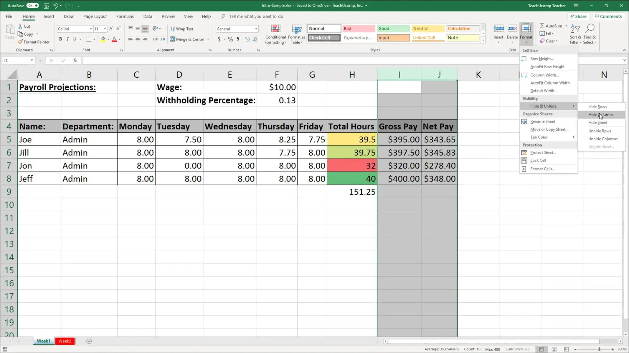
Go to the “Home” tab and click on the “Format” option in the “Cells” group.
From the dropdown menu, select “Hide Columns”. The selected columns will be hidden instantly.
To unhide the hidden columns, select the adjacent columns on both sides of the hidden columns, right-click, and choose “Unhide”.

Using Shortcut Keys:

If you prefer using keyboard shortcuts, here’s how you can hide and unhide columns:

To hide columns, select the columns and press “Ctrl” + “0” (zero).
To unhide columns, select the adjacent columns on both sides of the hidden columns, press “Ctrl” + “Shift” + “0”.

Using the Ribbon:

Excel also provides a convenient shortcut on the ribbon to hide and unhide columns. Follow these steps:

Select the column or columns that you want to hide or unhide.
Go to the “Home” tab and find the “Format” group.
Click on the “Hide & Unhide” button.
From the dropdown menu, choose either “Hide Columns” or “Unhide Columns” depending on your requirement.

Tips and Tricks:

Here are some additional tips and tricks for hiding and unhiding columns in Excel:

If you want to hide multiple columns, hold down the “Ctrl” key and select the desired columns before applying the hide command.
To quickly hide or unhide all columns in the worksheet, select the entire worksheet by clicking on the triangle at the intersection of row headers and column headers, then use the hide or unhide command.
If you frequently hide and unhide certain columns, you can customize the Quick Access Toolbar and add the hide and unhide commands for easy access.

Now that you know various methods to hide and unhide columns in Excel, you can efficiently manage your data and present it in a more organized way. Experiment with these techniques and explore the different ways to enhance your Excel skills.

How to Hide and Unhide Rows in Excel

Managing large datasets in Excel often requires the ability to hide and unhide rows. Whether you want to focus on specific information or create a cleaner view of your spreadsheet, hiding and unhiding rows can be incredibly useful. In this article, we will explore different methods to hide and unhide rows in Excel.

Using the Format Menu:

The easiest way to hide or unhide a row in Excel is by utilizing the Format menu. Follow these simple steps:

Select the row or rows that you want to hide. You can do this by clicking on the row number.
Go to the “Home” tab and click on the “Format” option in the “Cells” group.
From the dropdown menu, select “Hide Rows”. The selected rows will be hidden instantly.
To unhide the hidden rows, select the adjacent rows above and below the hidden rows, right-click, and choose “Unhide” from the context menu.

Using Shortcut Keys:

If you prefer using keyboard shortcuts, here is how you can hide and unhide rows:

To hide rows, select the rows and press “Ctrl” + “9”.
To unhide rows, select the adjacent rows above and below the hidden rows, press “Ctrl” + “Shift” + “9”.

Using the Ribbon:

Excel also provides a convenient option on the ribbon to hide and unhide rows. Follow these steps:

Select the row or rows that you want to hide or unhide.
Go to the “Home” tab and find the “Format” group.
Click on the “Hide & Unhide” button.
From the dropdown menu, choose either “Hide Rows” or “Unhide Rows” depending on your requirement.

Tips and Tricks:

Here are some additional tips and tricks for hiding and unhiding rows in Excel:

If you want to hide multiple rows, hold down the “Ctrl” key and select the desired rows before applying the hide command.
To quickly hide or unhide all rows in the worksheet, select the entire worksheet by clicking on the triangle at the intersection of row headers and column headers, then use the hide or unhide command.
If you frequently hide and unhide certain rows, you can customize the Quick Access Toolbar and add the hide and unhide commands for easy access.

Now that you know various methods to hide and unhide rows in Excel, you can efficiently manage your data and present it in a more organized and structured way. Explore these techniques to enhance your Excel proficiency and make data analysis a breeze.

How to Hide and Unhide Cells in Excel

In Microsoft Excel, there are times when you may want to hide specific cells to either simplify your worksheet or protect sensitive information. Excel provides various methods to hide and unhide cells, giving you control over what is visible and what remains hidden. In this article, we will explore different techniques for hiding and unhiding cells in Excel.

Using Cell Formatting:

The easiest way to hide a cell in Excel is by changing its cell format. Follow these steps:

Select the cell or cells you want to hide.
Right-click on the selected cell(s) and choose “Format Cells” from the context menu.
Go to the “Number” tab and choose “Custom” from the Category list.
In the “Type” field, enter ;;; (three semicolons) and click “OK”.
The selected cell(s) will now appear blank, effectively hidden.

To unhide the hidden cells, select the cell(s) adjacent to the hidden cells, right-click, and choose “Format Cells”. In the “Number” tab, select the desired format and click “OK”. The previously hidden cells will now be visible again.

Using Cell Protection:

If you want to hide cells and prevent them from being edited, you can use cell protection. Here’s how:

Select the cell(s) you want to hide.
Right-click and choose “Format Cells” from the context menu.
Go to the “Protection” tab and check the box that says “Hidden”. Click “OK”.
Next, go to the “Review” tab, click on “Protect Sheet” and enter a password.
The selected cells will now be hidden and protected. To unhide the cells, unprotect the sheet and remove the cell protection.

Using Conditional Formatting:

If you want to hide cells based on certain criteria, you can utilize conditional formatting. Here’s how:

Select the cell(s) you want to hide based on a condition.
Go to the “Home” tab and click on “Conditional Formatting”. Choose “New Rule”.
Select “Use a formula to determine which cells to format”.
In the “Format values where this formula is true” field, enter a formula that evaluates to TRUE for the cells you want to hide.
Set the formatting options to be the same as the background color.
Click “OK” to apply the conditional formatting.

The selected cells will now be hidden based on the specified condition. To unhide the cells, remove the conditional formatting from the cells.

Tips and Tricks:

Here are some additional tips for hiding and unhiding cells in Excel:

If you need to hide multiple cells, select the cells and apply one of the above methods.
To hide entire rows or columns, you can use the respective hiding methods mentioned earlier in this article.
If you frequently hide and unhide specific cells, you can create a shortcut by recording a macro that performs the necessary actions.

Now that you are familiar with different methods of hiding and unhiding cells in Excel, you can effectively manage your data and protect sensitive information. Explore these techniques to enhance your Excel skills and improve the organization of your spreadsheets.

Using the Format Menu to Hide and Unhide Columns, Rows, and Cells

Microsoft Excel provides a user-friendly interface with various options for hiding and unhiding columns, rows, and cells. One of the simplest methods to accomplish this is by using the Format menu. In this article, we will learn how to hide and unhide columns, rows, and cells using the Format menu in Excel.

Hiding Columns:

To hide a column using the Format menu, follow these steps:

Select the column or columns that you want to hide by clicking on the column header(s).
Go to the “Home” tab and find the “Cells” group.
Click on the “Format” option to open the dropdown menu.
Select “Hide Columns”. The selected columns will now be hidden from view.

Unhiding Columns:

To unhide columns using the Format menu, follow these steps:

Select the adjacent columns on both sides of the hidden columns to include them in the selection.
Go to the “Home” tab, click on the “Cells” group, and select “Format” from the dropdown menu.
Choose “Unhide Columns” to reveal the hidden columns.

Hiding Rows:

To hide a row using the Format menu, follow these steps:

Select the row or rows that you want to hide by clicking on the row number(s).
Go to the “Home” tab and find the “Cells” group.
Click on the “Format” option to open the dropdown menu.
Select “Hide Rows”. The selected rows will now be hidden from view.

Unhiding Rows:

To unhide rows using the Format menu, follow these steps:

Select the adjacent rows above and below the hidden rows to include them in the selection.
Go to the “Home” tab, click on the “Cells” group, and select “Format” from the dropdown menu.
Choose “Unhide Rows” to reveal the hidden rows.

Hiding Cells:

To hide individual cells in Excel using the Format menu, follow these steps:

Select the cell or cells that you want to hide by clicking on them.
Right-click on the selected cell(s) and choose “Format Cells” from the context menu.
Go to the “Number” tab and choose “Custom” from the Category list.
In the “Type” field, enter ;;; (three semicolons) and click “OK”. The selected cell(s) will now appear blank, effectively hidden.

Note: To unhide cells hidden using the format option, follow the same steps mentioned above and change the cell format to the desired type.

Using the Format menu in Excel to hide and unhide columns, rows, and cells provides a straightforward way to manage the visibility of specific data. Experiment with these techniques to customize your worksheets and present your data in a way that best suits your needs.

Using the Shortcut Keys to Hide and Unhide Columns, Rows, and Cells

Microsoft Excel offers a range of keyboard shortcuts to quickly hide and unhide columns, rows, and cells. These shortcuts provide a convenient and efficient way to manage the visibility of specific data in your worksheets. In this article, we will explore the commonly used shortcut keys to hide and unhide columns, rows, and cells in Excel.

Hiding Columns:

To hide columns using shortcut keys, follow these steps:

Select the column or columns that you want to hide by clicking on the column header(s).
Press “Ctrl” + “0” (zero) on your keyboard. The selected columns will be hidden instantly.

Unhiding Columns:

To unhide columns using shortcut keys, follow these steps:

Select the adjacent columns on both sides of the hidden columns to include them in the selection.
Press “Ctrl” + “Shift” + “0” on your keyboard. The hidden columns will be revealed.

Hiding Rows:

To hide rows using shortcut keys, follow these steps:

Select the row or rows that you want to hide by clicking on the row number(s).
Press “Ctrl” + “9” on your keyboard. The selected rows will be hidden instantly.

Unhiding Rows:

To unhide rows using shortcut keys, follow these steps:

Select the adjacent rows above and below the hidden rows to include them in the selection.
Press “Ctrl” + “Shift” + “9” on your keyboard. The hidden rows will be revealed.

Hiding Cells:

To hide individual cells using shortcut keys, follow these steps:

Select the cell or cells that you want to hide by clicking on them.
Right-click on the selected cell(s) and choose “Format Cells” from the context menu.
Go to the “Number” tab and choose “Custom” from the Category list.
In the “Type” field, enter ;;; (three semicolons) and click “OK”. The selected cell(s) will now appear blank, effectively hidden.

Note: To unhide cells hidden using the format option, right-click on the hidden cell, choose “Format Cells,” and change the cell format to the desired type.

Using shortcut keys is a time-saving technique to hide and unhide columns, rows, and cells in Excel. Incorporate these shortcuts into your workflow to efficiently manage the visibility of your data and enhance your productivity.

Using the Ribbon to Hide and Unhide Columns, Rows, and Cells

Microsoft Excel provides a convenient ribbon interface that allows you to easily hide and unhide columns, rows, and cells. The ribbon provides an intuitive visual menu, making it simple to manage the visibility of your data. In this article, we will explore how to use the ribbon to hide and unhide columns, rows, and cells in Excel.

Hiding Columns:

To hide columns using the ribbon, follow these steps:

Select the column or columns that you want to hide by clicking on the column header(s).
Go to the “Home” tab on the ribbon.
In the “Cells” group, click on the “Format” button to expand the menu.
From the dropdown menu, click on the “Hide & Unhide” option.
Select “Hide Columns” from the expanded menu. The selected columns will now be hidden.

Unhiding Columns:

To unhide columns using the ribbon, follow these steps:

Select the adjacent columns on both sides of the hidden columns to include them in the selection.
Go to the “Home” tab on the ribbon and click on the “Format” button in the “Cells” group.
From the dropdown menu, click on the “Hide & Unhide” option.
Select “Unhide Columns” from the expanded menu. The hidden columns will be revealed.

Hiding Rows:

To hide rows using the ribbon, follow these steps:

Select the row or rows that you want to hide by clicking on the row number(s).
Go to the “Home” tab on the ribbon.
In the “Cells” group, click on the “Format” button to expand the menu.
From the dropdown menu, click on the “Hide & Unhide” option.
Select “Hide Rows” from the expanded menu. The selected rows will now be hidden.

Unhiding Rows:

To unhide rows using the ribbon, follow these steps:

Select the adjacent rows above and below the hidden rows to include them in the selection.
Go to the “Home” tab on the ribbon and click on the “Format” button in the “Cells” group.
From the dropdown menu, click on the “Hide & Unhide” option.
Select “Unhide Rows” from the expanded menu. The hidden rows will be revealed.

Hiding Cells:

To hide cells using the ribbon, follow these steps:

Select the cell or cells that you want to hide by clicking on them.
Right-click on the selected cell(s) and choose “Format Cells” from the context menu.
Go to the “Number” tab and choose “Custom” from the Category list.
In the “Type” field, enter ;;; (three semicolons) and click “OK”. The selected cell(s) will now appear blank, effectively hidden.

Note: To unhide cells hidden using the format option, right-click on the hidden cell, choose “Format Cells,” and change the cell format to the desired type.

The ribbon in Excel provides a user-friendly interface for hiding and unhiding columns, rows, and cells. Incorporate the ribbon commands into your workflow to efficiently manage the visibility of your data and enhance your productivity.

Hiding and Unhiding Multiple Columns, Rows, and Cells

In Excel, there are often instances where you need to hide or unhide multiple columns, rows, or cells at once. This can save you time and effort, especially when working with large datasets. In this article, we will explore how to efficiently hide and unhide multiple columns, rows, and cells in Excel.

Hiding Multiple Columns:

To hide multiple columns simultaneously, follow these steps:

Select the first column you want to hide by clicking on its header.
Hold down the “Ctrl” key and continue selecting the additional columns. You can also drag your cursor across the column headers to make a continuous selection.
Once all the desired columns are selected, use one of the methods mentioned earlier, such as the Format menu or shortcut keys, to hide the selected columns.

Unhiding Multiple Columns:

To unhide multiple columns at once, follow these steps:

Select the columns adjacent to the hidden columns to include them in the selection.
Apply the unhide method you prefer, such as using the Format menu or shortcut keys, to reveal the hidden columns.

Hiding Multiple Rows:

If you need to hide multiple rows simultaneously, follow these steps:

Select the first row you want to hide by clicking on its row number.
Hold down the “Shift” key and continue selecting the additional rows. Alternatively, you can click and drag your cursor across the row numbers to create a continuous selection.
Once all the desired rows are selected, use one of the methods mentioned earlier, such as the Format menu or shortcut keys, to hide the selected rows.

Unhiding Multiple Rows:

To unhide multiple rows at once, follow these steps:

Select the rows adjacent to the hidden rows to include them in the selection.
Apply the unhide method of your choice, such as using the Format menu or shortcut keys, to reveal the hidden rows.

Hiding Multiple Cells:

If you want to hide multiple cells, irrespective of their location, follow these steps:

Select the first cell you want to hide.
Hold down the “Ctrl” key and continue selecting the additional cells. You can also drag your cursor across the cells to make a continuous selection.
Once all the desired cells are selected, use the method of your choice, such as changing the cell format or applying conditional formatting, to hide the selected cells.

Unhiding Multiple Cells:

To unhide multiple cells simultaneously, follow these steps:

Select the adjacent cells surrounding the hidden cells to include them in the selection.
Apply the method you used to hide the cells, such as changing the cell format or removing the conditional formatting, to reveal the hidden cells.

By utilizing these techniques, you can efficiently hide and unhide multiple columns, rows, and cells, allowing you to organize and manage your data more effectively in Excel.

Hiding and Unhiding Columns, Rows, and Cells with Specific Values

In Excel, you may encounter scenarios where you want to hide or unhide specific columns, rows, or cells based on their values. This can be particularly useful when you want to focus on certain data or filter out specific information. In this article, we will explore how to hide and unhide columns, rows, and cells with specific values in Excel.

Hiding Columns with Specific Values:

To hide columns with specific values, you can use Excel’s Autofilter feature. Follow these steps:

Select the column or columns that you want to filter.
Go to the “Data” tab on the ribbon and click on the “Filter” button.
Click on the filter arrow in the column header and choose “Filter by Color” or “Text Filters”.
Specify the criteria for hiding the columns based on their values.
Only the columns containing the specified values will be hidden.

Unhiding Columns with Specific Values:

To unhide columns with specific values that were previously hidden using Autofilter, follow these steps:

Remove the filter by clicking on the filter arrow in the column header and selecting “Clear Filter” or “Show All”.
All the hidden columns with specific values will now be revealed.

Hiding Rows with Specific Values:

To hide rows with specific values, you can use Excel’s Filter feature. Here’s how:

Select the range of cells or columns that you want to filter.
Go to the “Data” tab on the ribbon and click on the “Filter” button.
Click on the filter arrow in the column that contains the values you want to filter.
Specify the criteria for hiding the rows based on their values.
Only the rows containing the specified values will be hidden.

Unhiding Rows with Specific Values:

To unhide rows with specific values that were previously hidden using the Filter feature, follow these steps:

Remove the filter by clicking on the filter arrow in the column header and selecting “Clear Filter” or “Show All”.
All the hidden rows with specific values will now be revealed.

Hiding Cells with Specific Values:

To hide individual cells with specific values, you can use conditional formatting. Here’s how:

Select the range of cells that you want to apply conditional formatting to.
Go to the “Home” tab on the ribbon and click on the “Conditional Formatting” button.
Select “New Rule” and choose “Use a formula to determine which cells to format”.
Enter the formula that evaluates to TRUE for the cells you want to hide.
Specify the formatting options to hide the values (e.g., setting font color to match the background).

Unhiding Cells with Specific Values:

To unhide cells with specific values that were previously hidden using conditional formatting, follow these steps:

Remove the conditional formatting by going to the “Home” tab, clicking on the “Conditional Formatting” button, and selecting “Clear Rules” or “Clear Rules from Selected Cells”.
All the hidden cells with specific values will now be revealed.

By utilizing these techniques, you can easily hide and unhide columns, rows, and cells with specific values in Excel, allowing you to focus on the data that matters most to you.

Hiding and Unhiding Columns, Rows, and Cells in Filtered Data

When working with filtered data in Excel, you may need to hide or unhide columns, rows, or cells that are not currently visible due to the applied filter. Hiding and unhiding in filtered data helps you focus on specific information and manipulate your data more effectively. In this article, we will explore how to hide and unhide columns, rows, and cells in filtered data using Excel.

Hiding Columns in Filtered Data:

To hide columns in filtered data, follow these steps:

Apply the desired filter to your data by selecting the column header and going to the “Data” tab on the ribbon.
Once the filter is applied, select the columns you want to hide.
Right-click on one of the selected columns and choose “Hide” from the context menu.
The hidden columns will be removed from the visible data.

Unhiding Columns in Filtered Data:

To unhide columns in filtered data, follow these steps:

Clear the filter by going to the “Data” tab and clicking on the “Clear” button in the “Sort & Filter” group.
All the hidden columns will be revealed along with the filtered data.
Select the previously hidden columns and right-click on any of the selected columns.
Choose “Unhide” from the context menu to make the columns visible again.

Hiding Rows in Filtered Data:

To hide rows in filtered data, follow these steps:

Apply the desired filter to your data using the appropriate column.
Select the rows you want to hide.
Right-click on one of the selected rows and choose “Hide” from the context menu.
The hidden rows will be removed from the visible data.

Unhiding Rows in Filtered Data:

To unhide rows in filtered data, follow these steps:

Clear the filter by going to the “Data” tab and clicking on the “Clear” button in the “Sort & Filter” group.
All the hidden rows will be revealed along with the filtered data.
Select the previously hidden rows and right-click on any of the selected rows.
Choose “Unhide” from the context menu to make the rows visible again.

Hiding Cells in Filtered Data:

To hide specific cells in filtered data, follow these steps:

Apply the desired filter to your data using the appropriate column.
Select the cells you want to hide.
Right-click on one of the selected cells and choose “Format Cells” from the context menu.
In the “Format Cells” dialog box, go to the “Number” tab.
Select the “Custom” category and enter ;;; (three semicolons) in the “Type” field.
Click “OK” to apply the custom format, hiding the selected cells from view.

Unhiding Cells in Filtered Data:

To unhide cells in filtered data, follow these steps:

Clear the filter by going to the “Data” tab and clicking on the “Clear” button in the “Sort & Filter” group.
All the hidden cells will be revealed along with the filtered data.
Select the previously hidden cells and right-click on any of the selected cells.
Choose “Format Cells” from the context menu.
In the “Format Cells” dialog box, change the cell format to the desired type.
Click “OK” to make the cells visible again.

By utilizing these techniques, you can effectively hide and unhide columns, rows, and cells even in filtered data, allowing you to analyze and manipulate your data with more precision and ease.

Hiding and Unhiding Columns, Rows, and Cells in Protected Sheets

Excel provides the ability to protect sheets to prevent accidental changes to important information. However, you may still need to hide or unhide columns, rows, or cells within a protected sheet for specific purposes. In this article, we will explore how to hide and unhide columns, rows, and cells in protected sheets in Excel.

Hiding Columns in Protected Sheets:

To hide columns in a protected sheet, follow these steps:

Select the column or columns you want to hide.
Right-click on the selected columns and choose “Hide” from the context menu.
Click on the “Review” tab on the ribbon and then click on “Protect Sheet”.
Enter a password to protect the sheet and choose your desired protection options.
Click “OK” to apply the sheet protection.
The selected columns will now be hidden, and the sheet will remain protected.

Unhiding Columns in Protected Sheets:

To unhide columns in a protected sheet, follow these steps:

Right-click on any column header and choose “Unhide” from the context menu.
Enter the password you set for sheet protection.
Select the hidden columns you want to unhide.
Click “OK” to unhide the selected columns within the protected sheet.

Hiding Rows in Protected Sheets:

To hide rows in a protected sheet, follow these steps:

Select the row or rows you want to hide.
Right-click on the selected rows and choose “Hide” from the context menu.
Apply sheet protection by going to the “Review” tab and clicking on “Protect Sheet”.
Enter a password and choose the desired protection options.
Click “OK” to protect the sheet.
The selected rows will be hidden, and the sheet will remain protected.

Unhiding Rows in Protected Sheets:

To unhide rows in a protected sheet, follow these steps:

Right-click on any row header and choose “Unhide” from the context menu.
Enter the password set for sheet protection.
Select the hidden rows you want to unhide.
Click “OK” to unhide the selected rows within the protected sheet.

Hiding Cells in Protected Sheets:

To hide cells in a protected sheet, follow these steps:

Select the cell or cells you want to hide.
Right-click on the selected cells and choose “Format Cells” from the context menu.
Go to the “Protection” tab and check the box that says “Hidden”.
Apply sheet protection by clicking on “Protect Sheet” in the “Review” tab.
Enter a password and choose the desired protection options.
Click “OK” to protect the sheet.
The selected cells will be hidden, and the sheet will be protected.

Unhiding Cells in Protected Sheets:

To unhide cells in a protected sheet, follow these steps:

Right-click on any cell and choose “Format Cells” from the context menu.
Go to the “Protection” tab and uncheck the box that says “Hidden”.
Enter the password you set for sheet protection.
Select the hidden cells you want to unhide.
Click “OK” to unhide the selected cells within the protected sheet.

By using these techniques, you can effectively hide and unhide columns, rows, and cells within a protected sheet in Excel, providing flexible control over your data while maintaining the necessary level of security.

Hiding and Unhiding Columns, Rows, and Cells in Grouped Data

In Excel, you can use the grouping feature to organize and condense your data by collapsing and expanding groups of columns or rows. While working with grouped data, you may need to hide or unhide specific columns, rows, or cells within those groups. In this article, we will explore how to hide and unhide columns, rows, and cells in grouped data in Excel.

Hiding Columns in Grouped Data:

To hide columns in grouped data, follow these steps:

Select the columns you want to hide.
Right-click on the selected columns and choose “Hide” from the context menu.
The selected columns will be hidden within the group.

Unhiding Columns in Grouped Data:

To unhide columns in grouped data, follow these steps:

Select the columns adjacent to the hidden columns to include them in the selection.
Right-click on the selected columns and choose “Unhide” from the context menu.
The previously hidden columns will be revealed within the group.

Hiding Rows in Grouped Data:

To hide rows in grouped data, follow these steps:

Select the rows you want to hide.
Right-click on the selected rows and choose “Hide” from the context menu.
The selected rows will be hidden within the group.

Unhiding Rows in Grouped Data:

To unhide rows in grouped data, follow these steps:

Select the rows adjacent to the hidden rows to include them in the selection.
Right-click on the selected rows and choose “Unhide” from the context menu.
The previously hidden rows will be revealed within the group.

Hiding Cells in Grouped Data:

To hide cells in grouped data, follow these steps:

Select the cells you want to hide.
Right-click on the selected cells and choose “Format Cells” from the context menu.
Go to the “Protection” tab and check the box that says “Hidden”.
The selected cells will be hidden within the group.

Unhiding Cells in Grouped Data:

To unhide cells in grouped data, follow these steps:

Right-click on any cell and choose “Format Cells” from the context menu.
Go to the “Protection” tab and uncheck the box that says “Hidden”.
The previously hidden cells will be revealed within the group.

Note: It is important to keep in mind that hiding or unhiding columns, rows, or cells within a group affects the visibility within that specific group only. Any groups expanded or collapsed will still maintain the grouping structure.

By using these techniques, you can efficiently hide and unhide columns, rows, and cells within grouped data in Excel, providing a more organized and concise view of your data while retaining the flexibility to access specific details as needed.

Tips and Tricks for Hiding and Unhiding Columns, Rows, and Cells

Hiding and unhiding columns, rows, and cells in Excel can significantly improve the organization and presentation of your data. To help you make the most of this feature, here are some handy tips and tricks:

1. Use Shortcut Keys: Memorize the shortcut keys for hiding and unhiding columns (Ctrl+0 and Ctrl+Shift+0) or rows (Ctrl+9 and Ctrl+Shift+9). These shortcuts can save you time when working with large datasets.

2. Combine Multiple Selections: To hide or unhide multiple columns, rows, or cells simultaneously, hold down the “Ctrl” key while selecting the desired columns, rows, or cells. This makes it easier to apply changes to multiple areas at once.

3. Select the Entire Worksheet: To hide or unhide all columns or rows in one go, click on the intersection of the row and column headers (the gray square in the top-left corner). Then use the appropriate hide or unhide command.

4. Customize the Quick Access Toolbar: Add the hide and unhide commands to the Quick Access Toolbar for quick and easy access. Simply right-click on the toolbar, select “Customize Quick Access Toolbar,” and choose the hide and unhide commands from the list.

5. Apply Consistent Formatting: When hiding cells, consider formatting them with a consistent cell color or font color that matches the background. This ensures that hidden cells are not accidentally modified or overlooked.

6. Document Hidden Columns, Rows, or Cells: To keep track of your hidden elements, create a separate section or sheet where you note down the details of hidden columns, rows, or cells. This can be useful for future reference or when sharing the workbook with others.

7. Use Filters and Sorting: In addition to hiding and unhiding, utilize Excel’s filter and sorting capabilities to further organize and analyze your data. Filters allow you to selectively show or hide specific values, while sorting allows you to arrange data in a desired order.

8. Be Mindful of Protected Sheets: When working with protected sheets, ensure that you unprotect the sheet before attempting to hide or unhide columns, rows, or cells. Once changes are made, you can reapply the sheet protection to maintain data integrity.

9. Undo Hiding: If you mistakenly hide columns, rows, or cells, use the “Undo” command (Ctrl+Z) to revert the changes. It is a quick and convenient way to restore the visibility of hidden elements.

10. Practice Caution with Shared Workbooks: Be cautious when using hiding and unhiding features in shared workbooks, as these changes may affect the visibility of information for all users. Make sure to communicate any hiding or unhiding actions to colleagues to avoid confusion or data inconsistency.

By keeping these tips and tricks in mind, you can effectively hide and unhide columns, rows, and cells in Excel to maximize productivity and enhance data presentation.