How To Add, Hide, Freeze, Or Remove Columns In Sheets

Adding a Column

Adding a column to a spreadsheet can help you organize your data more efficiently and make it easier to analyze. Whether you need to insert a new column for additional data, or rearrange the order of existing columns, Google Sheets provides a simple and straightforward process.

To add a column in Google Sheets, follow these steps:

1. Select the column adjacent to where you want to insert the new column. For example, if you want to add a column between column B and C, select column C.
2. Right-click on the selected column header. A context menu will appear.
3. Click on the “Insert 1 above” or “Insert 1 below” option, depending on where you want to add the column.

Alternatively, you can also use keyboard shortcuts to add a column:

• For Windows and Chrome OS: Press Ctrl + Alt + = to add a column above the selected column, or Ctrl + Alt + – to add a column below.
• For Mac: Press Cmd + Option + = to add a column above, or Cmd + Option + – to add a column below.

Once you have added the column, you can rename the column header by double-clicking on it and typing the desired name. You can also enter data in the new column and perform calculations or apply formulas as needed.

Adding columns is a useful feature in Google Sheets that allows you to customize and modify your spreadsheet to meet your specific needs. Whether you are working on a simple budget or a complex data analysis, adding columns will help you visualize and manipulate your data more effectively.

Now that you know how to add a column in Google Sheets, let’s move on to the next section where we will explore how to hide a column.

Hiding a Column

Hiding a column in Google Sheets can be beneficial when you want to declutter your spreadsheet or temporarily remove certain data from view. It allows you to focus on specific columns or analyze data without distractions. The process of hiding a column in Google Sheets is straightforward and can be done in just a few simple steps.

To hide a column in Google Sheets, follow these steps:

1. Select the column or columns you want to hide by clicking on the column header(s). To select multiple columns, hold down the Ctrl key (Windows) or Cmd key (Mac) while clicking on the column headers.
2. Right-click on the selected column header(s) to open the context menu.
3. Click on the “Hide column” option from the context menu.

You can also use a keyboard shortcut to hide a column:

• For Windows and Chrome OS: Press Ctrl + Shift + 0 to hide the selected column(s).
• For Mac: Press Cmd + Shift + 0 to hide the selected column(s).

Once you have hidden a column, it will no longer be visible in the spreadsheet. However, any formulas or data associated with the hidden column will remain intact. This means that hiding a column doesn’t delete or remove any data—it simply hides it from view.

To unhide a hidden column, follow these steps:

1. Click and drag to select the columns on both sides of the hidden column.
2. Right-click on any of the selected column headers to open the context menu.
3. Click on the “Unhide columns” option from the context menu.

You can also unhide a hidden column using the following keyboard shortcut:

• For Windows and Chrome OS: Press Ctrl + Shift + 9 to unhide the column(s).
• For Mac: Press Cmd + Shift + 9 to unhide the column(s).

Hiding columns in Google Sheets provides flexibility and allows you to customize your spreadsheet to focus on the most relevant information. It is an excellent way to streamline your data and enhance your productivity. Now that you know how to hide columns in Google Sheets, we’ll move on to the next section where we’ll explore how to freeze a column.

Freezing a Column

In Google Sheets, freezing a column keeps it visible on the screen even when you scroll horizontally, allowing you to always have important information or headers in view. This is especially useful when working with large datasets or when analyzing data that spans across multiple columns.

To freeze a column in Google Sheets, follow these steps:

1. Select the column to the right of the column you want to freeze. For example, if you want to freeze column A, select column B by clicking on the column header.
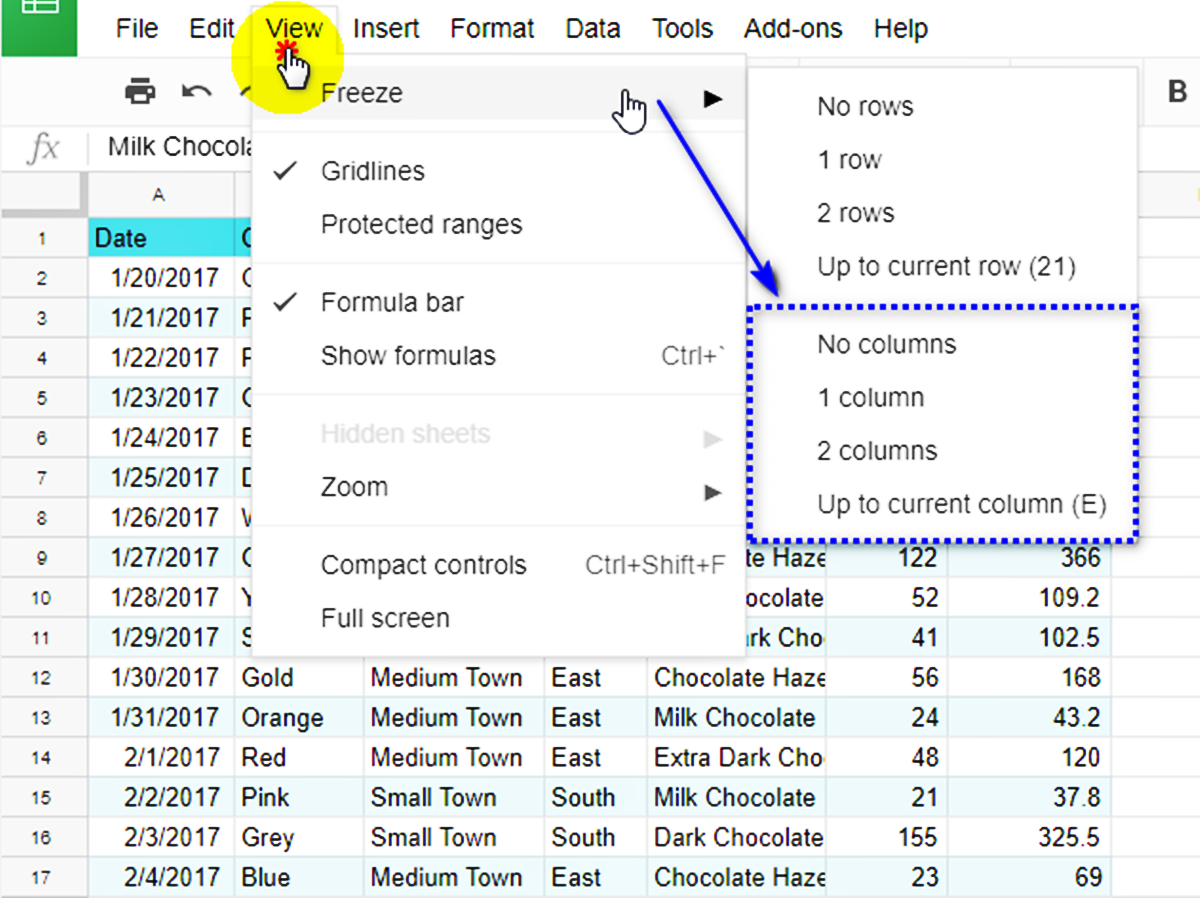
2. Click on the View menu at the top of the screen.
3. From the drop-down menu, select Freeze, then choose 1 column.

Alternatively, you can use a keyboard shortcut to freeze a column:

• For Windows and Chrome OS: Press Ctrl + Alt + F, followed by C.
• For Mac: Press Cmd + Option + F, followed by C.

Once you have frozen a column, you will notice a gray line appearing to the right of the frozen column. This indicates that the column is now frozen, and when you scroll horizontally, the frozen column will remain visible while the other columns move.

To unfreeze a column, follow these steps:

1. Click on the View menu at the top of the screen.
2. From the drop-down menu, select Freeze, then choose No rows.

Alternatively, you can use the following keyboard shortcut:

• For Windows and Chrome OS: Press Ctrl + Alt + F, followed by N.
• For Mac: Press Cmd + Option + F, followed by N.

Freezing columns in Google Sheets helps you maintain visibility of important data while scrolling through large spreadsheets. It allows you to focus on specific information and makes data analysis more convenient. Now that you know how to freeze columns, let’s move on to the next section where we’ll explore how to remove a column.

Removing a Column

At times, you may need to remove a column from your Google Sheets spreadsheet to reorganize data or simplify the layout. Removing a column ensures that any associated data or formatting is deleted as well. Google Sheets provides an easy process to remove a column, allowing you to adjust your spreadsheet as needed.

To remove a column in Google Sheets, follow these steps:

1. Select the entire column by clicking on the column header. For instance, if you want to remove column C, click on the “C” header.
2. Right-click on the column header to open the context menu.
3. Click on the “Delete column” option from the context menu.

You can also use a keyboard shortcut to remove a column:

• For Windows and Chrome OS: Press Ctrl + – to delete the selected column.
• For Mac: Press Cmd + – to delete the selected column.

Once you remove a column, the data in the column and any associated formulas or formatting will be permanently deleted. It’s important to be cautious when removing columns, as this action cannot be undone.

If you accidentally remove a column, you can use the “Undo” command by pressing Ctrl + Z (Windows/Chrome OS) or Cmd + Z (Mac) immediately to restore the deleted column.

Removing a column in Google Sheets allows you to restructure your spreadsheet and tailor it to your specific needs. By removing unnecessary columns, you can keep your data organized and focus on the most relevant information. Remember to exercise caution when removing columns to avoid accidentally deleting essential data.

Now that you’ve learned how to remove a column, you have a comprehensive understanding of how to add, hide, freeze, and remove columns in Google Sheets. These features provide you with the flexibility and control to customize your spreadsheet and effectively manage your data.