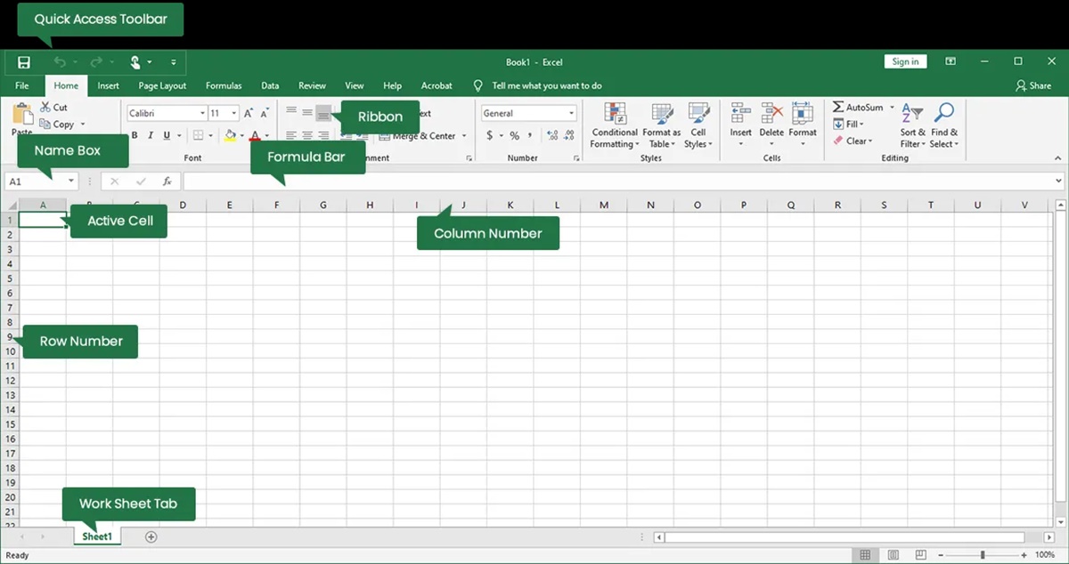
Understand the Basic Excel Screen Elements

Excel Ribbon

The Excel Ribbon is an essential part of Microsoft Excel’s interface. It is a strip that runs across the top of the Excel window, containing a collection of tabs, each with its own set of commands and tools. The Ribbon is designed to provide easy access to the various features and functions that Excel has to offer, making it more efficient for users to navigate and perform tasks.

Within the Excel Ribbon, there are several tabs, such as Home, Insert, Page Layout, Formulas, Data, Review, and View. Each tab is organized into groups, which logically group related commands together. For example, the Home tab typically includes commands for formatting cells, applying styles, and editing data.

One of the advantages of the Ribbon is that it displays contextual tabs and commands based on the task or object selected. This means that when you click on a specific feature or object, such as a chart or a table, additional tabs and options related to that object will appear in the Ribbon, providing quick access to relevant functions.

Customization options are also available in the Ribbon. Users can add their own tabs, groups, and commands to create a custom Ribbon tailored to their specific needs. This allows for a more personalized and efficient Excel experience.

Navigating the Ribbon is straightforward. You can either click on the desired tab to access its commands, or you can use Alt key shortcuts to bring up the associated keystrokes for each tab and command. The Ribbon is also designed to adapt to different screen sizes, ensuring that it remains accessible and functional on various devices.

Quick Access Toolbar

The Quick Access Toolbar is a customizable toolbar located above the Excel Ribbon. It provides quick and easy access to commonly used commands, tools, and functions, regardless of the active tab or context. By default, the Quick Access Toolbar includes commands such as Save, Undo, and Redo, but users have the flexibility to add or remove commands as desired.

The advantage of the Quick Access Toolbar is that it allows users to save time by having their most frequently used commands readily available. This can be especially helpful for repetitive tasks or actions that are performed frequently during spreadsheet work. Adding a command to the Quick Access Toolbar is as simple as right-clicking on the command in the Ribbon or selecting the command from the dropdown menu, and choosing “Add to Quick Access Toolbar”.

The placement of the Quick Access Toolbar above the Ribbon ensures that it is always visible, regardless of the active tab. This means that users can access their preferred commands without having to navigate through different tabs. Furthermore, users can customize the position of the Quick Access Toolbar, either by keeping it above the Ribbon or moving it below, depending on their personal preference.

In addition to adding commands from the Ribbon, the Quick Access Toolbar also provides direct access to other Excel features, such as custom macros or add-ins. This allows users to create shortcuts for specific functions or tools that are not readily available in the Ribbon.

The Quick Access Toolbar can be customized further by adjusting its display options. Users can choose to display the toolbar with text labels, icons only, or a combination of both. This flexibility ensures that users can optimize the toolbar’s appearance to suit their individual needs and preferences.

Overall, the Quick Access Toolbar serves as a convenient and efficient way to access frequently used commands in Excel. Its customization options and constant visibility make it a valuable tool for streamlining workflow and improving productivity.

Excel Worksheet

An Excel worksheet is the main working area within Microsoft Excel, where data is entered, manipulated, and analyzed. It consists of a grid of cells arranged in rows and columns, forming a table-like structure. Each cell can contain various types of data, such as numbers, text, or formulas.

One of the key features of an Excel worksheet is its ability to perform calculations and data analysis. Users can enter formulas into cells to perform mathematical operations or create complex calculations. Excel provides a wide range of built-in functions that make it easy to perform calculations, such as SUM, AVERAGE, and COUNT.

The grid-like structure of the worksheet allows for efficient organization and manipulation of data. Users can insert, delete, and rearrange rows and columns as needed to accommodate data or create meaningful layouts. Additionally, formatting options, such as font styles, cell borders, and background colors, can be applied to enhance the visual appearance of the worksheet.

Excel offers various tools and features to aid in data entry and management. Users can use auto-fill to quickly populate cells with a series of numbers, dates, or other patterns. Sorting and filtering options allow for easy data analysis and organization. Conditional formatting can be applied to highlight specific data based on certain conditions.

An Excel worksheet can also be used to create charts and graphs to visually represent data in a more understandable format. Users can select the data range and choose from a variety of chart types, including bar charts, line charts, and pie charts. Customization options are available to modify the appearance and layout of the charts.

Collaboration and sharing are facilitated through Excel worksheets. Multiple users can work on the same worksheet simultaneously, making real-time updates and edits. Users can protect and secure worksheets by setting passwords or restricting certain actions, ensuring data integrity and privacy.

Cell

In Excel, a cell is a fundamental unit within a worksheet and is identified by a unique combination of a column letter and a row number. It is where data can be entered, stored, and manipulated. The intersection of a column and a row creates a cell.

A cell can contain different types of data such as numbers, text, dates, and formulas. By default, the content of a cell is aligned to the right, and numbers are usually right-aligned while text is left-aligned. Cells can be formatted to display data in different formats, such as currency, percentages, or date formats, providing flexibility and customization.

Data in cells can be edited by simply selecting the cell and entering new values or text. Excel also offers various data validation options, allowing users to set specific criteria or restrictions on the type of data that can be entered into a cell. This helps maintain data accuracy and consistency.

One of the powerful features of Excel is its ability to perform calculations using formulas. Formulas can be entered directly into the cells to perform mathematical operations or manipulate data. When a formula is entered into a cell, Excel automatically recalculates the result whenever the data in the referenced cells is changed. This allows for dynamic and efficient data analysis.

Cells can reference other cells, creating dependencies between them. This means that the value or content of one cell can depend on the value or content of another cell. This is particularly useful when building complex calculations or performing data analysis, as it allows for the creation of interconnected formulas.

Excel provides additional features for working with cells, such as merging cells to create a larger, combined cell, splitting merged cells, and adjusting the width and height of cells to accommodate different data or formatting needs. Cells can also be formatted with cell borders, background colors, and font styles to improve readability and visual appeal.

The ability to select and manipulate cells in Excel is fundamental to working with data effectively. Users can select individual cells, ranges of cells, or even entire columns and rows to perform actions such as copying, pasting, formatting, or deleting. The versatility and functionality of cells make Excel a powerful tool for data organization and analysis.

Column

In Excel, a column refers to the vertical arrangement of cells from top to bottom within a worksheet. Columns are identified by letters at the top of the worksheet, starting with column A and continuing with subsequent letters as you move to the right.

Columns in Excel serve as a way to organize and categorize data. They provide a structured layout that allows users to store and analyze information in a tabular format. Each column can contain different types of data, such as numbers, text, or dates.

One of the main benefits of using columns in Excel is the ability to perform calculations and functions on a range of cells within a column. Users can apply mathematical operations, formulas, or built-in functions to calculate totals, averages, and other data analysis measures. This makes it easier to manipulate and analyze data across a large dataset.

Columns can be customized to suit specific data needs. Excel provides various formatting options for columns, including adjusting the width of a column to accommodate different data or applying specific number or text formats. Users can also freeze columns to keep them visible while scrolling through large sets of data, ensuring important information remains in view.

When working with columns, it is possible to insert or delete entire columns within a worksheet. This allows users to add or remove data columns as needed, rearranging the layout or adjusting the organization of the data. Deleting a column also removes all the data within that column, so caution should be exercised to avoid unintentional data loss.

Columns can also be grouped together in Excel, allowing users to collapse or expand multiple columns as a single entity. This is useful for organizing and managing large datasets, as it provides a way to hide or reveal specific sections of data, making it easier to focus on relevant information.

Excel provides functions and tools specific to working with columns. Users can sort and filter data within a column, making it easier to find and analyze specific information. They can also apply conditional formatting to highlight cells that meet certain criteria, improving data visualization and analysis. Additionally, users can reference data from different columns when creating formulas or performing complex calculations.

Columns play a critical role in organizing, manipulating, and analyzing data within Excel. Their versatility and functionality make them a vital component for effectively managing and interpreting information in a spreadsheet.

Row

In Excel, a row refers to the horizontal arrangement of cells from left to right within a worksheet. Rows are identified by numbers along the left side of the worksheet, starting with row 1 and continuing with subsequent numbers as you move down.

Rows in Excel are used to organize and structure data in a tabular format. Each row represents a record or entry, containing various types of data such as numbers, text, or dates. Rows serve as the foundation for storing and manipulating information within a worksheet.

One of the primary benefits of using rows in Excel is their ability to store and manipulate data in a structured manner. Users can enter values, formulas, or functions into cells within a row to perform calculations or generate results based on the data contained in that row.

Rows can be customized to fit specific data requirements. Excel offers various formatting options for rows, including adjusting the height of a row to accommodate different font sizes or adding specific cell borders to separate rows visually. This allows for better organization and readability of data.

In Excel, users can insert or delete rows within a worksheet. This functionality is particularly useful when new data needs to be added or when existing data needs to be rearranged. When a row is deleted, all the data within that row is removed as well.

Excel provides several features and functions specific to working with rows. Users can sort and filter data within a row to easily locate and analyze information. They can also apply conditional formatting to highlight cells that meet specific criteria, making it easier to identify patterns or trends within a row.

Rows can be grouped together in Excel, allowing users to collapse or expand multiple rows as a single entity. This feature is helpful when organizing and managing large datasets, as it allows for hiding or revealing specific sections of data, making it easier to focus on relevant information.

When working with rows, users can reference data from different rows when creating formulas or performing calculations. This enables the ability to perform calculations across multiple rows, such as calculating totals or averages.

Rows play a crucial role in organizing, manipulating, and analyzing data within Excel. Their flexibility and functionality make them essential for effectively managing and interpreting information in a spreadsheet.

Name Box

The Name Box is a feature in Microsoft Excel that allows users to view and manipulate cell references or define names for cells, ranges, or formulas. It is located towards the left of the formula bar, above the worksheet grid.

By default, the Name Box displays the current cell reference, indicating the column letter and row number of the active cell. It serves as a quick reference tool to easily determine the position of the selected cell within the worksheet.

The Name Box is also used to define names for individual cells or ranges, which can then be used in formulas and functions. This allows users to assign a meaningful name to a specific cell or range, making it easier to understand the purpose or context of the data when working with complex formulas or large datasets.

To define a name using the Name Box, users can first select the cell or range they want to name and then type the desired name directly into the Name Box. Once a name is assigned, it can be used in formulas by typing the name instead of the cell reference. This not only simplifies formula creation but also improves the readability and maintainability of the spreadsheet.

The Name Box also offers functionality beyond cell referencing. Users can click on the drop-down arrow within the Name Box to view a list of existing names defined within the workbook. This makes it easy to see all the defined names at a glance and quickly jump to the associated cell or range.

Furthermore, the Name Box can be used to navigate to specific cells or ranges within a worksheet. By typing the name or cell reference into the Name Box and pressing Enter, Excel will automatically select the corresponding cell or range, allowing for efficient navigation within the workbook.

In addition to cell references and named ranges, the Name Box can display other useful information. For example, when a calculation is in progress, the Name Box may display “Calculating” to indicate that Excel is still processing the data.

The Name Box is a versatile tool in Excel that provides various functions, including displaying cell references, defining names for cells or ranges, and facilitating navigation within a workbook. Its intuitive interface and practical features enhance the usability and productivity of working with Excel spreadsheets.

Formula Bar

The Formula Bar is a prominent feature in Microsoft Excel that appears directly above the worksheet grid. It is an essential tool for entering, editing, and viewing formulas and data within cells.

When a cell is selected in Excel, its contents, whether it be data or a formula, are displayed in the Formula Bar. This area allows users to see and manipulate the content in a larger, more convenient space compared to the limited size of the cell itself.

The Formula Bar provides a user-friendly interface for entering formulas. By clicking on the Formula Bar, users can directly type formulas or enter mathematical operations, cell references, and functions. This feature allows for precise control over calculations and data manipulation.

Excel’s Formula Bar also offers error checking capabilities. If a formula is entered incorrectly or encounters an error during calculation, an error message or indicator will be displayed in the Formula Bar. This helps users identify and correct formula errors, ensuring accurate and reliable calculations.

Users can easily edit and modify formulas using the Formula Bar. By selecting a cell containing a formula, the Formula Bar displays the full formula, allowing users to make adjustments and revisions as needed. This feature is particularly useful when working with complex formulas or making changes across multiple cells.

The Formula Bar also supports autocompletion, which assists users in entering functions and referring to cell ranges. As users begin typing a function or cell reference, a dropdown menu appears, suggesting available options based on what has been entered. Users can select options from this menu, reducing the chance of typographical errors and providing efficiency in formula creation.

Another convenient feature of the Formula Bar is the ability to view and edit long text within cells. If a cell contains a significant amount of text, only a portion may be visible within the cell itself. However, the Formula Bar allows users to view, edit, and manipulate the entire text within the selected cell.

The Formula Bar can also be resized or customized based on user preferences. Users can adjust the height of the Formula Bar to accommodate more lines of text or allow for easier reading of lengthy formulas.

Overall, the Formula Bar in Excel plays a vital role in entering, editing, and viewing formulas and data within cells. Its user-friendly interface, error-checking capabilities, editing functionality, and support for complex calculations make it an indispensable tool for working with mathematical calculations and data manipulation within Excel.

Sheet Tabs

In Microsoft Excel, sheet tabs are the tabs located at the bottom of the Excel window that represent individual worksheets within a workbook. They allow users to navigate and switch between different sheets within the same workbook.

Sheet tabs are labeled with default names such as “Sheet1,” “Sheet2,” and so on, but they can be renamed to provide a more descriptive title that reflects the contents or purpose of the sheet. Users can right-click on a sheet tab, select “Rename,” and enter a new name for the sheet.

Sheet tabs make it easy to manage and organize data within a workbook. Each sheet functions as an independent workspace, allowing users to separate and categorize information. This is especially useful for large datasets or when working on different aspects or scenarios of a project.

Users can add and delete sheet tabs as needed. Excel allows for a large number of sheets within a single workbook, so users can create and switch between multiple sheets to efficiently organize their data and analysis. Adding a new sheet tab can be done by right-clicking on an existing sheet tab and selecting “Insert,” or by using the designated button for inserting new sheets.

Sheet tabs also offer a range of additional functionality. Users can easily copy or move worksheets within a workbook by dragging and dropping the sheet tabs to their desired location. This feature allows for quick reordering of sheets or creating duplicate sheets for different purposes.

Formatting options are available for sheet tabs as well. Users can change the color of sheet tabs to differentiate between related sheets or to highlight important sheets. This can be done by right-clicking on a sheet tab, selecting “Tab Color,” and choosing a preferred color from the palette.

Sheet tabs can also be used to facilitate navigation and selection within a workbook. By holding down the Ctrl key and clicking on multiple sheet tabs, users can select and work with multiple sheets simultaneously. This allows for easy editing or formatting across selected sheets.

Additionally, Excel provides shortcuts and features to streamline sheet tab navigation. Users can utilize the “Ctrl+Page Up” and “Ctrl+Page Down” keyboard shortcuts to move between adjacent sheet tabs. The right-click menu on a sheet tab also offers options to navigate to any sheet within the workbook by selecting the desired sheet name from the list.

Scroll Bars

In Excel, scroll bars are vertical and horizontal bars that appear on the right side and bottom of the worksheet window, respectively. They provide a means to navigate and view different areas of a worksheet that cannot fit within the visible portion of the screen.

The vertical scroll bar allows users to move up and down within the worksheet, while the horizontal scroll bar enables left and right movement. By clicking and dragging the scroll bar handle, users can scroll through the worksheet in the corresponding direction, revealing hidden data or moving to a different area of the spreadsheet.

Scroll bars become particularly useful when dealing with large worksheets that contain more data than can be displayed on the screen. Users can effortlessly scroll through rows or columns to access cells that are not currently visible, making it easy to work with extensive spreadsheets.

Excel allows for customization of scroll bars to suit individual preferences. Users can right-click on a scroll bar and select “Scroll Bar Options” to adjust attributes such as the size, behavior, or appearance of the scroll bar. This includes modifying the scroll bar’s width, length, or its ability to increment smoothly or in fixed steps.

In addition to the scroll bar handles, Excel provides other scroll bar components to enhance the navigation experience. The arrow buttons at each end of the scroll bars allow for small incremental movements in the respective direction. Clicking on these buttons moves the view of the worksheet up, down, left, or right by a fixed amount.

Excel also offers the scroll bar page buttons, which are found immediately above and below the scroll bar handle in the vertical scroll bar and to the left and right of the horizontal scroll bar handle. Clicking on these buttons moves the view one page up, down, left, or right, allowing for larger jumps within the worksheet.

In addition to scrolling vertically and horizontally, users can use both scroll bars together to navigate diagonally within a worksheet. By clicking and dragging on the intersection of the vertical and horizontal scroll bars, users can move in any direction while maintaining the same view proportions.

Scroll bars are not limited to their default positions. Users can adjust the scroll area of a worksheet by setting it to a specific range of cells. This allows for precise control of the visible portion of the worksheet and enables users to focus on specific areas of interest.

Overall, scroll bars in Excel provide an intuitive and efficient way to navigate through large worksheets, making it easy to access and work with data that extends beyond the visible screen area. With their customization options and various components, scroll bars offer flexibility and enhanced user experience in Excel.

Status Bar

The Status Bar is a horizontal bar located at the bottom of the Excel window. It provides useful information and tools that assist users in working with the worksheet and performing various tasks.

The Status Bar displays different types of information depending on the context or user actions. By default, it shows the current status of the worksheet, such as Ready or Editing, indicating whether the user can interact with the worksheet or is currently entering data or making edits.

One of the primary functions of the Status Bar is to provide quick access to important settings and features. Users can right-click on the Status Bar to enable or disable various options, such as displaying the average, count, or sum of selected cells, or the page number when viewing multiple worksheets.

The Status Bar also includes tools and indicators that provide information about the current selection. For example, it shows the number of selected cells, as well as the sum, average, minimum, and maximum values of the selected range.

Excel’s Status Bar offers additional features to aid in data analysis and manipulation. For example, when multiple worksheets are selected, it provides a tab count, allowing users to quickly determine the number of selected sheets. When the AutoSum feature is used, the Status Bar displays the sum of the selected cells or the adjacent cells if no selection is made.

The Status Bar provides real-time updates for specific actions or tasks. For instance, when pressing the Caps Lock key, the Status Bar displays the “Caps Lock on/off” indicator, alerting users to the current state of the Caps Lock key. This helps users avoid unintended text entry when the Caps Lock key is activated.

Users can customize the elements that appear on the Status Bar to suit their needs. By right-clicking on the Status Bar, users can choose the desired options from the context menu, such as adding or removing specific functions or indicators.

In addition to its default features, the Status Bar can also provide insights relevant to specific tasks or actions performed in Excel. For example, when entering or editing a formula, the Status Bar displays information about the error status of the formula, indicating if there are any issues or inconsistencies.

The Status Bar in Excel serves as a multi-purpose tool that offers various functions and information to enhance the user experience. Its versatility, customization options, and real-time updates provide valuable insights and tools for effective data analysis and manipulation.

View Buttons

The View Buttons are a set of icons located in the bottom-right corner of the Excel window, next to the Zoom Slider. They provide quick access to different viewing options and settings that allow users to customize the appearance and layout of the worksheet.

These buttons offer various views to suit different needs and preferences. Let’s explore the different functions of the View Buttons:

Normal View: This is the default view in Excel. It displays the worksheet in a clean and straightforward layout, showing the gridlines, columns, and rows as they appear in the printed version.
Page Layout View: This view provides a more accurate representation of how the worksheet will appear when printed. It shows the headers, footers, margins, and page breaks, allowing users to adjust the layout and formatting accordingly.
Page Break Preview: This view helps users visualize and manipulate page breaks within the worksheet. It displays dashed lines to indicate the page boundaries and allows users to drag and adjust the page breaks to control how the worksheet will be divided and printed.
Full Screen View: This view expands Excel to fill the entire screen, providing a distraction-free workspace. It removes the ribbon and other elements from the screen, allowing users to focus solely on the worksheet.

In addition to these primary views, the View Buttons also offer other options and features:

Split Window: This feature divides the Excel window into multiple panes, allowing users to scroll within each pane separately. It is useful for comparing data, referencing information in different parts of the worksheet, or working with large datasets.
Freeze Panes: This option enables users to lock specific rows or columns in place while scrolling through the worksheet. It ensures that critical information remains visible and easily accessible even when navigating through large sets of data.

The View Buttons provide flexibility and convenience in customizing the way data is presented and viewed within Excel. Users can easily switch between different views and access additional features to enhance their workflow and analysis of the worksheet.

Zoom Slider

The Zoom Slider is a tool located in the bottom-right corner of the Excel window, adjacent to the View Buttons. It allows users to adjust the magnification level of the worksheet, making it larger or smaller for easier viewing.

The Zoom Slider provides a quick and convenient way to change the zoom level. By default, the slider is set to 100%, which displays the worksheet at its normal size, with one cell equal to one pixel on the screen. Moving the slider to the right increases the zoom percentage, making the content larger and more visible, while moving it to the left reduces the zoom percentage, shrinking the content for a wider view of the worksheet.

The Zoom Slider offers flexibility in customizing the display of the worksheet. It allows users to zoom in to get a closer look at small details or zoom out to see a broader view of the entire worksheet. The visual representation of the slider makes it easy to see the current zoom level at a glance.

In addition to using the Zoom Slider, users can also zoom in or out by using other methods:

Zoom Control: Clicking on the “+” or “-” buttons located next to the Zoom Slider adjusts the zoom level incrementally.
Zoom Dialog Box: Clicking on the Zoom Slider itself opens a dialog box where users can enter a specific zoom percentage or choose from predefined options.
Keyboard Shortcuts: Using keyboard shortcuts, such as Ctrl + “+” (plus) to zoom in or Ctrl + “-” (minus) to zoom out, allows users to quickly adjust the zoom level without using the mouse.

The Zoom Slider is particularly useful when working with large or complex spreadsheets, as it makes it easier to read and navigate the content. Users can zoom in to focus on specific details or zoom out to get an overview of the entire worksheet.

Excel also allows users to set a custom zoom level as the default view. This feature ensures that every time the workbook is opened, it will display at the preferred zoom level set by the user, providing a consistent viewing experience.

The Zoom Slider provides a user-friendly and efficient way to adjust the magnification level of the worksheet in Excel. It offers flexibility in customizing the view and allows users to adapt the display to suit their needs, improving readability and ease of use within the spreadsheet.

Navigation Buttons

The Navigation Buttons in Excel are a set of buttons located to the left of the Zoom Slider in the bottom-right corner of the Excel interface. They provide a convenient way to navigate between different worksheets within a workbook.

The Navigation Buttons consist of two arrows, one pointing to the left and the other to the right. These buttons allow users to move sequentially through the worksheets in a workbook, either in a forward or backward direction, similar to flipping through the pages of a book.

By clicking the right-facing arrow, users can move to the next worksheet in the workbook. This is useful when working with multiple sheets and wanting to quickly switch to the next sheet without going back to the sheet tabs at the bottom of the screen.

Conversely, clicking the left-facing arrow allows users to navigate to the previous worksheet. This is beneficial when needing to review or edit earlier sheets within the workbook and retrace steps in the workflow.

In addition to using the Navigation Buttons for linear navigation, users can also access individual sheets directly by right-clicking on either button. This action will display a list of all the sheets within the workbook, allowing users to select the desired sheet to navigate to.

The Navigation Buttons provide a convenient method for moving between sheets and improve the efficiency of working within a workbook. They eliminate the need to locate and click on specific sheet tabs, which can be time-consuming when dealing with a large number of sheets or when sheets are not displayed in one visible row.

One advantage of the Navigation Buttons is their accessibility and ease of use. Even if the sheet tabs are hidden due to limited space on the screen, the Navigation Buttons remain visible and accessible for swift navigation.

It is important to note that the Navigation Buttons are specific to navigating between sheets within a single workbook. To switch between different workbooks, users would need to use alternative methods, such as utilizing the taskbar or the “Switch Windows” option in the View tab of the Ribbon.

The Navigation Buttons provide a quick and efficient way to move through worksheets in Excel. Being easily accessible and eliminating the need to locate specific sheet tabs, they enhance user productivity and streamline workflow when working with multiple sheets within a workbook.

Split Window

The Split Window feature in Excel allows users to divide the worksheet window into multiple panes, providing a convenient way to view and work with different parts of the worksheet simultaneously. It is particularly useful when dealing with large datasets or when comparing information from different areas within the same worksheet.

To activate the Split Window feature, users can go to the View tab in the Ribbon and click on the “Split” button. Alternatively, they can use the keyboard shortcut of Alt + W + S.

Once the Split Window feature is enabled, the worksheet window is split into separate panes. Users can adjust the position of the split by clicking and dragging the gray divider bar that appears. This allows for creating multiple horizontal or vertical panes depending on the desired layout.

The Split Window feature offers several benefits:

Simultaneous Viewing: With the split window, users can simultaneously view different sections of the worksheet. This makes it easy to compare data, reference information in one section while working in another, or navigate through complex spreadsheets more efficiently.
Independent Scrolling: Each pane within the split window can be scrolled independently of the others. This enables users to navigate through different parts of the worksheet while keeping other sections in view, making it easier to locate and analyze data.
Freezing Panes: Users can combine the Split Window feature with the Freeze Panes option to keep specific rows or columns visible while scrolling through other sections of the worksheet. This is especially useful when working with large amounts of data, as it allows users to focus on important information while retaining context.

To remove the split, users can use the “Remove Split” button in the View tab of the Ribbon or the keyboard shortcut of Alt + W + P. This restores the worksheet to its normal view.

The Split Window feature provides a flexible and efficient way to work with large datasets or compare information within a worksheet. By enabling simultaneous viewing and independent scrolling, it enhances productivity and improves the usability of Excel when working with complex spreadsheets.

Worksheet Views

Excel offers various worksheet views that allow users to customize how the worksheet is displayed, making it easier to work with and analyze data. These different views provide flexibility and versatility, catering to different user requirements and preferences.

Let’s explore some of the key worksheet views available in Excel:

Normal View: This is the default view in Excel, displaying the worksheet with all its elements, including headers, footers, gridlines, and data. It provides a standard and straightforward view for data entry and general editing.
Page Layout View: This view presents the worksheet as it would appear when printed, allowing users to see the layout, margins, headers, footers, and other page-specific elements. It aids in fine-tuning the appearance and formatting of the worksheet for printing purposes.
Page Break Preview: This view assists users in managing page breaks within the worksheet. It displays dashed lines indicating page boundaries, making it easier to adjust and control how the worksheet will be divided and printed across multiple pages.
Full Screen View: This view maximizes the Excel window, occupying the entire screen space. It hides the ribbon, formula bar, and other distractions, providing a focused and distraction-free environment for working with the worksheet.
Custom Views: Custom views allow users to save and switch between different combinations of worksheet settings, such as zoom level, hidden columns or rows, filtered data, or print options. This enables users to quickly switch between different views tailored to specific needs or scenarios.

Each of these views serves a specific purpose and offers unique advantages. By switching between views, users can adapt the display of the worksheet to suit their current task or analysis requirements.

In addition to these default views, Excel also provides other view options, such as Draft view for editing the worksheet with simplified visuals or Split view for dividing the worksheet window into multiple panes for simultaneous viewing and scrolling.

Excel’s versatile worksheet views enhance productivity and improve the overall user experience by offering different perspectives and tailored displays for effective data management and analysis.

File Tab

The File tab is a central feature of Microsoft Excel, located in the top-left corner of the Excel window. It provides access to various commands and options related to managing and working with workbooks and documents.

When the File tab is clicked, it opens the Backstage view, a dedicated space that offers a range of functionality and tools for file management, customization, sharing, printing, and more.

The File tab features several key components:

New: This option allows users to create a new workbook from scratch or choose from a variety of built-in templates. It offers different templates for tasks such as budgeting, scheduling, calendars, and more, giving users a head start for specific projects.
Open: This command opens the Open dialog box, where users can browse and select existing workbooks to open or access recently opened workbooks conveniently from the list.
Save/Save As: These options enable users to save their current workbook to a desired location on the computer or network. The Save As option allows users to save the workbook with a new name or in a different file format if needed.
Print: This command opens the printing options, allowing users to manage the printing settings, choose the printer, adjust page layout, and preview the printed document before sending it to the printer.
Share: The Share option provides various ways to collaborate and share workbooks with others. Users can invite others to view or edit the workbook simultaneously, email the workbook as an attachment, or publish it to an online platform.
Options: This feature opens the Excel Options dialog box, where users can customize settings for Excel, including general options, formulas, proofing, data, and more. It provides a range of customization choices to tailor Excel to individual preferences.
Exit: This option allows users to exit Excel and close the application.

The File tab and Backstage view in Excel provide a centralized and comprehensive set of commands and options for managing workbooks, accessing templates, saving, printing, sharing, and customizing Excel’s settings. It serves as a hub for efficient file management and improved user productivity.

Backstage View

The Backstage view is an integral part of Microsoft Excel and is accessed by clicking on the File tab in the top-left corner of the Excel window. It provides a centralized and comprehensive space for managing workbooks, accessing various commands, and customizing Excel settings.

When the Backstage view is opened, it replaces the main worksheet area, allowing users to focus on file-related actions and settings. Here are some key features and options available within the Backstage view:

New: This section offers options to create a new workbook from scratch or choose from a wide range of built-in templates. Users can select templates for budgets, calendars, invoices, schedules, and more, providing a quick-start for their projects.
Open: This section allows users to browse and open existing workbooks from their computer, OneDrive, or other cloud storage platforms. It also provides quick access to recently opened workbooks, making it easy to resume work on previously accessed files.
Save / Save As: In this section, users can save their current workbook or save it with a different name or format using the Save As option. It also provides options to save the workbook to different locations, such as the computer, OneDrive, or other cloud storage services.
Print: The Print section allows users to configure printing settings, choose the printer, specify the number of copies, and preview the printed document. It provides various options to ensure accurate and efficient printing of the workbook.
Share: This section offers options for collaborating and sharing workbooks with others. Users can invite others to view or edit the workbook, email the workbook as an attachment, or publish it to Microsoft SharePoint or other online platforms.
Options: The Options section provides access to Excel’s settings and preferences. Here, users can customize various aspects of Excel, such as general settings, formulas, proofing, data, and add-ins. It allows users to tailor Excel to their specific needs and work preferences.
Exit: This option exits Excel and closes the application.

The Backstage view in Excel simplifies file management and enhances productivity by providing a centralized location for commonly used actions and settings related to workbooks. It offers a streamlined approach to create, open, save, print, share, and customize Excel files, saving users valuable time and effort.

Recent Workbooks

The Recent Workbooks feature in Excel provides quick access to the most recently opened workbooks, making it easier for users to resume their work and continue where they left off with just a few clicks.

Located in the Backstage view, the Recent Workbooks section displays a list of the most recently opened workbooks, including both local files and those stored in cloud storage services like OneDrive or SharePoint. The list is dynamically populated based on the user’s actions, ensuring that the most relevant and frequently accessed workbooks are readily available.

This feature offers several advantages:

Time-Saving: Instead of manually searching for a specific workbook in the file directory, users can simply access their recently opened workbooks from the list. This eliminates the need to remember file locations or navigate through multiple folders.
Efficient Workflow: The Recent Workbooks list promotes a seamless workflow by allowing users to quickly switch between different workbooks. This is especially beneficial when working on multiple projects or when collaborating with others on different files.
Convenience: As the list is updated automatically, users do not need to actively manage or maintain it. Excel keeps track of the workbooks accessed by the user, ensuring that the list remains up to date and reflects the most relevant and recent files.
Cloud Integration: The Recent Workbooks feature includes workbooks that are stored in cloud storage services like OneDrive or SharePoint. This allows users to access their files from any device with an internet connection, further enhancing mobility and collaboration.

Moreover, the Recent Workbooks list in Excel can be customized based on user preferences. Users can pin specific workbooks to the list, ensuring that important files remain easily accessible, even if they haven’t been recently accessed.

The Recent Workbooks feature streamlines the process of accessing recently used files in Excel, improving productivity and user experience. By reducing the time and effort required to locate and open workbooks, it enables users to work more efficiently and focus on their tasks without getting bogged down by file management.

Save and Open Documents

The ability to save and open documents is a fundamental feature in Excel that enables users to create, store, and access their workbooks and spreadsheets. With these capabilities, users can easily save their work, protect against data loss, and retrieve files for future use.

When working on a new or existing workbook in Excel, users can save their document by clicking on the File tab and selecting the “Save” or “Save As” command. Saving a document allows users to store their work on a local drive, in a specific folder, or in cloud storage. By assigning a name to the document, users can easily identify and retrieve it later.

During the saving process, users have the option to choose different file formats, depending on their needs. Excel supports various file formats such as Excel Workbook (.xlsx), Excel Macro-Enabled Workbook (.xlsm), or even older versions of Excel formats for compatibility purposes. Choosing the appropriate file format ensures compatibility with other versions of Excel and other spreadsheet software.

Excel also provides an “AutoSave” feature that automatically saves changes as users work, minimizing the risk of data loss in case of unexpected computer failure or interruption. This feature periodically saves the workbook in the background, offering peace of mind and convenience for users.

To access previously saved workbooks, users can click on the File tab and select the “Open” command. This action opens the Open dialog box, where users can browse their computer or cloud storage to locate and retrieve the desired workbook. Additionally, Excel also presents a list of recently opened workbooks in the Recent Workbooks section of the Backstage view, making it even more convenient to open frequently used files.

When opening a workbook, users can view a preview of the file to confirm it is the desired document before opening it. They can also filter the file list by file type, date modified, or search for a specific file by name.

In addition to traditional local storage, Excel supports integration with cloud storage services like OneDrive, Dropbox, or SharePoint. This allows users to save their workbooks in the cloud, providing the flexibility of accessing files from any device with an internet connection. It also promotes seamless collaboration and file sharing with others.

Overall, the ability to save and open documents in Excel is critical for document management, data preservation, and efficient workflow. It empowers users to save their work, conveniently retrieve files, and choose different file formats to ensure compatibility and accessibility across devices and software platforms.

Print Options

The print options in Excel provide users with a variety of settings and customization features to ensure that their worksheets and workbooks are printed accurately and efficiently. Excel offers a range of print options that allow users to control the appearance, layout, and other aspects of the printed document.

When users are ready to print their worksheet or workbook, they can click on the File tab and select the “Print” command. This opens the print options, allowing users to configure various settings:

Printer Selection: Users can choose the printer they want to use for printing their document. This is especially useful in environments with multiple printers or when users need to print documents on different types of paper or in different formats.
Page Orientation: Excel offers the option to print in either portrait or landscape mode. This setting determines whether the printed document will be taller or wider, depending on the orientation chosen. Users can select the desired orientation based on their specific needs and the layout of their worksheet.
Page Size: Users can specify the size of the paper on which their document will be printed. Excel offers a variety of standard page sizes, such as letter, legal, A4, and more. By selecting the appropriate page size, users can ensure that their content fits correctly on the printed page without any cropping or scaling issues.
Print Range: Users can define the specific range of cells or pages they want to print. This allows for selective printing, enabling users to print specific portions of a worksheet or only the pages they need. It can help conserve paper and improve efficiency when printing large or complex workbooks.
Print Preview: Excel provides a print preview feature, allowing users to see how their document will look when printed. This enables users to check for any layout or formatting issues before actually printing the document, saving time and resources.
Print Scaling: Excel offers the option to adjust the scale of the printed document. Users can specify a custom scaling percentage to make the content larger or smaller on the printed page, ensuring optimal readability and usability.

In addition to these options, Excel provides various other advanced print settings, including headers and footers, margins, gridlines, and more. These features allow users to further customize the appearance of the printed document, ensuring it meets their specific preferences and requirements.

The print options in Excel empower users to create professional, accurate, and customized printouts of their worksheets and workbooks. By providing flexibility and control over the printing process, Excel helps users optimize the presentation and usability of their data when transitioning from a digital to a physical format.

Options

The Options feature in Excel provides users with a wide range of settings and customization options to tailor the application to their needs and preferences. By accessing the Excel Options dialog box, users can modify various aspects of Excel’s behavior, appearance, functionality, and other important settings.

To access the Options dialog box, users can click on the File tab, select “Options,” and explore the available categories and settings. Here are some key areas where users can customize Excel:

General: In the General category, users can set preferences for displaying recent files, managing the Office Clipboard, specifying the default font, selecting the language, and more. This allows users to personalize Excel and tailor it to their specific working preferences.
Formulas: The Formulas category offers options related to formula calculations, error checking, and other formula-related settings. Users can choose to enable or disable automatic formula calculation, modify error checking rules, change how Excel handles cell references, and more.
Proofing: In the Proofing category, users can customize proofing tools such as spelling and grammar checking, autocorrection options, custom dictionaries, and language preferences. It allows users to fine-tune the proofing features to suit their specific language and writing needs.
Data: The Data category provides options related to external data connections, sorting and filtering, importing and exporting data, and other data-specific settings. Users can configure how Excel handles imported data, specify default sorting behavior, set data connection properties, and more.
Advanced: The Advanced category includes a wide range of advanced settings, such as display options, editing options, file options, formula options, and more. It allows users to fine-tune Excel’s behavior, control how data is displayed, set calculation options, adjust file-saving preferences, and customize other advanced features.

The Options dialog box provides users with granular control over their Excel experience, allowing them to adjust settings based on their specific requirements and working preferences. It empowers users to optimize Excel’s functionality, appearance, and behavior to enhance productivity and streamline their workflow.

Moreover, the Options dialog box often includes additional settings for add-ins, language preferences, trust center options, customization of the ribbon and Quick Access Toolbar, and more. This comprehensive range of customizable settings ensures that users can make Excel work seamlessly for their individual needs and maximize their efficiency and productivity.

Help and Support

The Help and Support feature in Excel provides users with a valuable resource to access assistance, obtain guidance, and troubleshoot issues when using the application. Excel offers multiple avenues for users to find answers to their questions and receive support to maximize their usage of the software.

Excel’s Help and Support feature comprises several elements to cater to users’ needs:

Help Center: Excel’s Help Center is a comprehensive repository of information and documentation. It includes a vast collection of articles, tutorials, how-to guides, and step-by-step instructions on various Excel topics. Users can access the Help Center by clicking on the “Help” button or searching for specific keywords.
Smart Lookup: Smart Lookup is an integrated feature that allows users to obtain additional context and definitions for highlighted words or phrases within Excel. By right-clicking on a term and selecting “Smart Lookup,” users can access relevant information from the web powered by Bing.
Online Community: Excel’s online community is made up of forums and discussion boards where users can interact with other Excel enthusiasts and experts. These communities allow users to ask questions, seek advice, and share knowledge. Microsoft’s official Excel community, as well as other third-party forums, can be valuable resources to find solutions to specific Excel-related challenges.
Microsoft Support: Microsoft provides official support channels where users can seek assistance directly from the company. Users can access Microsoft’s support website, submit a support request, or use virtual chat options to connect with Microsoft support professionals for guidance on technical issues, installation problems, or functionality clarification.
In-App Help: Excel also includes context-sensitive help features integrated within the application. Users can access these features by clicking on the “?” icon or the “Tell me what you want to do” box in the ribbon. This feature allows users to search for specific commands or actions and provides direct links to relevant Help Center articles.

Excel’s Help and Support resources offer users the tools and assistance they need to overcome challenges, discover additional features, and deepen their understanding of the software. The availability of these support options ensures that users can navigate Excel efficiently and make the most of its features.

Whether users prefer to explore the Help Center, engage with the online community, seek assistance directly from Microsoft, or utilize the in-app help features, Excel’s Help and Support capabilities empower users to find the answers and guidance they need to optimize their experience with the application.