Splitting the Screen in Excel

Why Split the Screen in Excel?

When working with large spreadsheets in Excel, it can be challenging to keep track of important data while navigating through different sections. This is where the “Split Screen” feature in Excel comes into play. Splitting the screen allows you to divide your worksheet into multiple panes, making it easier to view and compare data from different parts of the sheet without the need for scrolling back and forth.

One of the major advantages of splitting the screen in Excel is improved efficiency. By having multiple panes, you can simultaneously view different areas of your worksheet and perform tasks more quickly. This is particularly useful when you need to compare data from different sections or when you are working on a complex project that involves referencing multiple cells or ranges.

Another benefit of using the split screen feature is better data analysis. By segregating your worksheet into different panes, you can focus on specific areas of the sheet and analyze the data more effectively. This helps you identify patterns, trends, and anomalies without the distraction of unnecessary information.

Moreover, splitting the screen can enhance collaboration and teamwork. When working with colleagues or clients, it’s often necessary to discuss or review specific parts of a spreadsheet. By splitting the screen, you can share relevant information with others easily and have discussions while keeping everyone on the same page.

Furthermore, splitting the screen can be highly advantageous when dealing with large amounts of data. It allows you to maintain a fixed reference point while scrolling through extensive lists or tables. This ensures that essential information remains visible at all times, even when you’re working with vast datasets.

How to Split the Screen in Excel

Splitting the screen in Excel is a straightforward process that can be done in a few simple steps. Here’s how you can do it:

Select the cell in the worksheet where you want to split the screen. This will become the dividing point for the split screen.
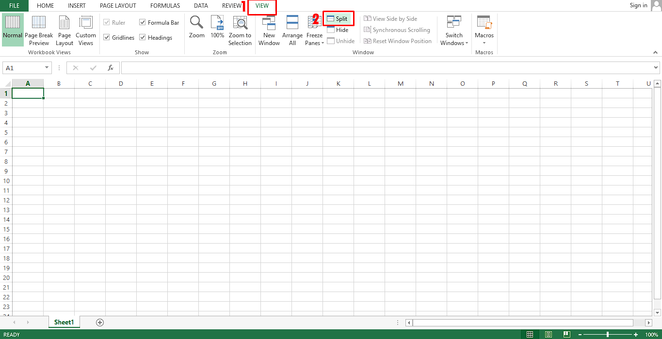
Go to the “View” tab in the Excel ribbon.
In the “Window” group, click on the “Split” button. This will immediately split the screen horizontally, with the selected cell as the dividing point.
If you want to split the screen vertically as well, place the cursor in the cell where you want the vertical splitting to occur.
Go to the “View” tab again and click on the “Split” button once more.
You will now have a split screen with both horizontal and vertical dividers.

You can adjust the size of each pane by clicking on the dividing line and dragging it to your desired position. This allows you to control the amount of data displayed in each section.

To remove the split from the screen, simply go to the “View” tab and click on the “Split” button to toggle off the split screen view.

It’s important to note that splitting the screen is a temporary view change and does not affect the actual structure or format of your Excel worksheet. When you close and reopen the file, the split screen will no longer be active, but you can easily recreate it using the steps mentioned above.

Now that you know how to split the screen in Excel, you can take advantage of this feature to enhance your productivity and data analysis capabilities.

Splitting the Screen Vertically

Splitting the screen vertically in Excel allows you to view and compare different columns or sections of your worksheet side by side. This can be especially useful when working with wide datasets or when you need to reference specific columns while entering data or performing calculations.

Here’s how you can split the screen vertically in Excel:

Select the cell in the worksheet where you want the vertical splitting to occur. This will become the dividing point for the split screen.
Go to the “View” tab in the Excel ribbon.
In the “Window” group, click on the “Split” button. This will split the screen horizontally by default, with the selected cell as the dividing point.
To split the screen vertically, place the cursor in the cell where you want the vertical splitting to occur.
Go to the “View” tab again and click on the “Split” button once more.
You will now have a split screen with both horizontal and vertical dividers, allowing you to view multiple columns simultaneously.

Once the screen is split vertically, you can adjust the position and size of each pane by clicking and dragging the vertical dividing line.

By splitting the screen vertically, you can easily compare data from different columns without the need to scroll horizontally. This makes it convenient to analyze and manipulate large datasets, identify correlations, and perform data entry tasks more efficiently.

Remember that the split screen view is temporary and can be removed by clicking on the “Split” button in the “View” tab. Additionally, you can resize the panes or remove the split by dragging the dividing lines to the desired positions.

Splitting the screen vertically in Excel is an invaluable technique for anyone working with extensive datasets or needing to compare columns in a worksheet. It helps improve productivity and reduces the time spent scrolling back and forth, allowing for seamless navigation and analysis of your data.

Splitting the Screen Horizontally

Splitting the screen horizontally in Excel is a useful feature that allows you to view and compare different rows or sections of your worksheet simultaneously. This can be particularly beneficial when working with large datasets or when you need to reference specific rows while entering or analyzing data.

Here’s how you can split the screen horizontally in Excel:

Select the cell in the worksheet where you want the horizontal splitting to occur. This will be the dividing point for the split screen.
Go to the “View” tab in the Excel ribbon.
In the “Window” group, click on the “Split” button. This will split the screen horizontally, with the selected cell as the dividing point.
If you want to split the screen vertically as well, place the cursor in the cell where you want the vertical splitting to occur.
Go to the “View” tab again and click on the “Split” button once more.
You will now have a split screen with both horizontal and vertical dividers, enabling you to view multiple rows simultaneously.

Once the screen is split horizontally, you can adjust the position and size of each pane by clicking and dragging the horizontal dividing line.

Splitting the screen horizontally allows you to compare data from different rows without the need to scroll vertically. This makes it convenient for analyzing and manipulating large datasets, identifying trends, and performing data entry tasks more efficiently.

It’s important to note that the split screen view is temporary and can be removed by clicking on the “Split” button in the “View” tab. You can also resize the panes or remove the split by dragging the dividing lines to the desired positions.

By splitting the screen horizontally in Excel, you can significantly improve your workflow and productivity when working with extensive data. It eliminates the need for constant scrolling, enhances data comparison, and enables easier navigation and analysis of your spreadsheet.

Removing the Split from the Screen

When you no longer need the split screen view in Excel, you can easily remove it to return to the normal viewing mode. Here’s how you can remove the split from the screen:

Go to the “View” tab in the Excel ribbon.
In the “Window” group, click on the “Split” button. This will toggle off the split screen view and merge the panes back into a single viewing area.

Alternatively, you can remove the split by clicking and dragging the dividing lines to the edge of the worksheet until they disappear.

It’s important to note that removing the split from the screen does not affect the structure or format of your Excel worksheet. It simply returns your view to the normal, unsplit state.

By removing the split, you regain full visibility of your worksheet and can continue working without any divided panes. This is particularly useful when you have finished referencing or analyzing data from different sections and want to focus on the entire spreadsheet.

Remember that removing the split does not undo any changes you made to your data while in the split screen view. It only changes the viewing mode back to a single, unsplit window.

Removing the split screen from Excel is quick and easy, allowing you to switch seamlessly between split and single view modes as needed for your tasks and analysis.

Navigating the Split Screen in Excel

Once you have split the screen in Excel, it’s important to know how to navigate within the split view to effectively work with your data. Here are some tips for navigating the split screen in Excel:

To scroll through the split panes, use the scroll bars that appear within each pane. You can scroll horizontally and vertically independently within each pane to view different sections of your worksheet.
To adjust the size of the panes, hover your mouse over the dividing line until it turns into a double-headed arrow. Then, click and drag the line to your desired position. You can resize the panes to allocate more space to specific sections of your worksheet.
If you want to switch focus between the panes, simply click inside the pane you want to work in. This will allow you to enter data, perform calculations, or select cells without affecting the other pane.
When working with formulas or data references, keep in mind that the cell references adjust automatically within each pane. For example, if you enter a formula in one pane that references a cell, it will adjust accordingly if you scroll to a different section in the other pane.
If you need to copy or move data between different sections of your worksheet, you can use the standard copy (Ctrl+C) and paste (Ctrl+V) commands. Excel will recognize the active pane and perform the desired operation accordingly.
To remove the split from the screen and return to the normal view, you can click on the “Split” button in the “View” tab, or drag the dividing lines to the edge of the worksheet until they disappear.

By familiarizing yourself with these navigation techniques, you can efficiently work with the split screen in Excel and easily access different sections of your worksheet.

Remember that the split screen view is temporary and doesn’t affect the structure or format of your Excel worksheet. You can always switch back to the normal view to work with the entire spreadsheet or remove the split altogether if it’s no longer needed.

Efficient navigation within the split screen allows you to analyze and manipulate data more effectively, saving you time and increasing your productivity when working with large datasets or complex spreadsheets.

Tips and Tricks for Using Split Screens in Excel

Split screens in Excel can greatly improve your productivity and efficiency when working with large datasets. Here are some tips and tricks to maximize your usage of the split screen feature:

Use freeze panes: In addition to splitting the screen, you can also freeze panes to keep certain rows or columns visible as you scroll. This is especially handy when you want to keep headers or labels in view while exploring different sections of a worksheet. Simply select the row below and the column to the right of where you want to freeze, and go to the “View” tab > “Freeze Panes” > “Freeze Panes”.
Use multiple split screens: Excel allows you to have multiple split screens open in the same workbook. This feature is particularly beneficial when you need to compare data from different worksheets or when you want to work on multiple sections simultaneously. Simply repeat the steps to split the screen for each section you want to view.
Save and restore split settings: If you frequently work with the split screen feature and want to save time setting it up, Excel allows you to save the split settings. After splitting the screen as desired, go to the “View” tab > “Window” group > “Arrange All” > “Vertical” or “Horizontal”. This will save the split settings which you can easily restore by using the “Arrange All” option again.
Maximize screen space: To maximize the workspace within each pane, consider hiding the ribbon and formula bar temporarily. This will provide more screen real estate for viewing and working with your data. To hide or show the ribbon and formula bar, go to the “View” tab and uncheck/check the “Formula Bar” and “Ribbon” options in the “Show/Hide” group.
Utilize keyboard shortcuts: Excel provides several keyboard shortcuts to work efficiently with split screens. For example, press Alt+W, M to maximize the active pane, Alt+W, S to split the screen, and Alt+W, Q to toggle the split screen on and off. Familiarize yourself with these shortcuts to save time and streamline your workflow.

By implementing these tips and tricks, you can make the most of the split screen feature in Excel and enhance your data analysis, comparison, and overall productivity.