How to Freeze Column and Row Headings in Excel

Why Freeze Column and Row Headings in Excel?

When working with large datasets in Excel, it can become challenging to keep track of column and row headings. These headings provide essential context and ensure data accuracy. However, as you scroll through hundreds or even thousands of rows and columns, these headings can easily disappear from view, causing confusion and potentially leading to errors.

By freezing column and row headings in Excel, you can overcome this hurdle and maintain a clear and structured view of your data. Freezing headings allows them to remain visible on the screen while you navigate through the spreadsheet, ensuring that you always have valuable reference points.

Freezing column and row headings offers several benefits:

Improved Navigation: With frozen headings, you can easily identify which data belongs to a particular column or row, making it efficient to navigate and understand complex spreadsheets.
Data Analysis: Freezing column and row headings enables you to compare and analyze data across different sections of a spreadsheet without losing track of the relevant headings.
Data Entry: By freezing row headings, you can minimize the chances of entering data in the wrong row, ensuring accurate data entry and reducing errors.
Presentation: When sharing Excel files, frozen headings maintain the structure and formatting, making it easier for others to understand and work with the data.
Efficient Printing: Freezing headings before printing helps maintain the visual integrity of the spreadsheet and ensures that the headings are included on each page.

Overall, freezing column and row headings in Excel is a valuable technique that improves data management, navigation, analysis, and presentation, ultimately enhancing productivity and accuracy in spreadsheet tasks.

How to Freeze Column Headings in Excel

Freezing column headings in Excel is a straightforward process that can greatly improve your data management experience. Here’s how you can do it:

Open your Excel spreadsheet and locate the row beneath the column headings that you want to freeze. This row should contain the data in your spreadsheet.
Click on the cell directly below the column headings that you want to freeze. This will be the first cell of your data.
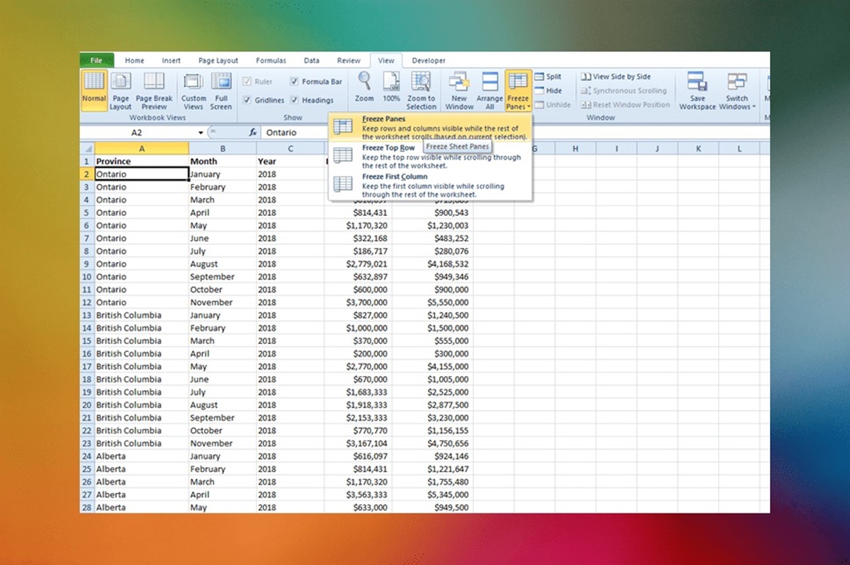
In the Excel menu, go to the “View” tab and click on the “Freeze Panes” option. A drop-down menu will appear.
From the drop-down menu, select the “Freeze Panes” option. Excel will freeze the selected row, ensuring that the column headings remain visible as you scroll through the spreadsheet.
Verify that the column headings are frozen by scrolling through the spreadsheet. You will notice that the frozen row stays in place while the rest of the data scrolls accordingly.

That’s it! You have successfully frozen the column headings in your Excel spreadsheet. Now, you can work with your data more efficiently without losing track of the column names.

It’s important to note that freezing column headings only affects the horizontal scrolling of your spreadsheet. If you want to freeze both column and row headings, continue reading to learn how.

How to Freeze Row Headings in Excel

In some cases, it may be more beneficial to freeze row headings instead of or in addition to freezing column headings in Excel. Freezing row headings ensures that the labels for each row remain visible as you navigate through the spreadsheet. Here’s how you can freeze row headings:

Open your Excel spreadsheet and locate the column to the right of the row headings that you want to freeze. This column should contain the data in your spreadsheet.
Select the column to the right of the row headings by clicking on the corresponding column letter at the top of the spreadsheet.
In the Excel menu, go to the “View” tab and click on the “Freeze Panes” option. A drop-down menu will appear.
From the drop-down menu, select the “Freeze Panes” option. Excel will freeze the selected column, ensuring that the row headings remain visible as you scroll through the spreadsheet.
Verify that the row headings are frozen by scrolling through the spreadsheet. You will notice that the frozen column stays in place while the rest of the data scrolls accordingly.

By freezing row headings, you can easily identify the category or description associated with each row, even when working with a large dataset. This can be especially useful when analyzing data or updating information in specific rows.

Remember, freezing row headings only affects the vertical scrolling of your spreadsheet. If you want to freeze both column and row headings for a complete freeze effect, continue reading to learn how to do it.

How to Freeze Both Column and Row Headings in Excel

If you want to maximize the benefits of freezing column and row headings in Excel, you can freeze both at the same time. This allows you to keep your column and row headings visible as you navigate through your spreadsheet. Here’s how you can freeze both column and row headings:

Open your Excel spreadsheet and locate the top-left cell of the data range that you want to freeze. This cell should be just below the row headings and to the right of the column headings.
Click on the cell to select it and ensure that it is the active cell.
In the Excel menu, go to the “View” tab and click on the “Freeze Panes” option. A drop-down menu will appear.
From the drop-down menu, select the “Freeze Panes” option. Excel will freeze both the selected row and column, ensuring that the column and row headings remain visible as you scroll through the spreadsheet.
Verify that both the column and row headings are frozen by scrolling through the spreadsheet. You will notice that the frozen row and column stay in place while the rest of the data scrolls accordingly.

By freezing both column and row headings, you can have a fixed reference point for your data, allowing for seamless data analysis, navigation, and data entry. This is especially useful when dealing with large datasets that require frequent scrolling.

Remember to adjust the freezing range if you need to freeze different rows or columns in your spreadsheet. Excel allows you to customize the freezing based on your specific needs.

Tips and Tricks for Freezing Headings in Excel

Now that you know how to freeze column and row headings in Excel, here are some additional tips and tricks to enhance your experience:

Adjust the Freeze Panes Range: If you need to freeze a different set of column or row headings, Excel allows you to adjust the freeze panes range. Simply select the cell below and to the right of the headings you want to freeze, and then go to the “View” tab and click on “Freeze Panes” again. Select the “Freeze Panes” option, and the new range will be frozen.
Unfreeze Panes: To remove the freezing effect and unfreeze panes in Excel, go to the “View” tab, click on “Freeze Panes,” and select “Unfreeze Panes.” This will unfreeze all frozen panes in your spreadsheet.
Use Split Panes: Instead of freezing panes, you can also use the “Split” feature in Excel to create separate, movable panes. This allows you to view different sections of your spreadsheet simultaneously. To split panes, go to the “View” tab, click on “Split,” and Excel will create a horizontal or vertical split at the active cell.
Combine Freeze Panes with Filter and Sort: You can use the freeze panes feature in combination with Excel’s filter and sort options to analyze and manage your data more effectively. Freeze the necessary panes and then apply filters or sorting to specific columns or rows for targeted data analysis.
Try Auto-Fit Column Width: When working with frozen column headings, Excel may not automatically adjust the column width based on the content. To ensure that the text in each column heading is fully visible, select the column(s) and double-click the right boundary of the selected column header. Excel will adjust the width to fit the content automatically.

By utilizing these tips and tricks, you can optimize your usage of frozen headings in Excel, enhancing your productivity, data management, and analysis capabilities.