
Why Freeze Rows or Columns?
Freezing rows or columns in Google Sheets can be incredibly helpful when working with large datasets or complex spreadsheets. It allows you to keep important information in view while scrolling through the rest of the data. By freezing certain rows or columns, you can ensure that important headers, labels, or formulas are always visible, no matter how far you scroll.
Here are three key benefits of freezing rows or columns:
- Easy Navigation: By freezing the top row or leftmost column, you can easily identify which data is associated with each column or row as you scroll through your sheet. This makes it quicker and more convenient to navigate and understand your spreadsheet, especially when dealing with large amounts of data.
- Data Analysis: Freezing rows or columns is essential for accurate analysis. When working with large datasets, freezing headers or labels allows you to always have a clear reference point. This ensures that you are referencing the correct data while performing calculations or creating data visualizations.
- Improved Readability: Freezing rows or columns can greatly enhance the readability of your spreadsheet. By keeping important information visible, you can avoid constant scrolling back and forth, making it easier to understand and interpret the data. This is particularly useful when sharing your spreadsheet with others.
Overall, by freezing rows or columns, you can maintain the context, structure, and readability of your spreadsheet, making it easier to work with and analyze the data.
How to Freeze Rows or Columns in Google Sheets
Freezing rows or columns in Google Sheets is a straightforward process. Follow these steps to freeze specific rows or columns in your spreadsheet:
Step 1: Select the Row or Column to Freeze
Start by opening your spreadsheet in Google Sheets. Identify the row or column that you want to freeze. Click on the number of the row or the letter of the column to select it.
Step 2: Access the Freeze Menu
Next, go to the “View” menu at the top of the Google Sheets interface. Click on it to expand the menu options.
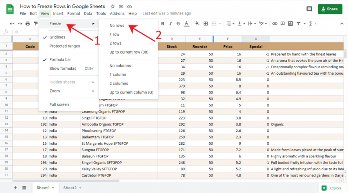
Step 3: Choose the Freeze Option
In the “View” menu, hover your cursor over the “Freeze” option. A submenu will appear with different freezing options:
- Freeze 1 row: This option will freeze the selected row at the top of the spreadsheet, keeping it visible while scrolling vertically.
- Freeze 2 rows: This option will freeze the selected row and the row below it at the top of the spreadsheet.
- Freeze 1 column: This option will freeze the selected column at the left-most side of the spreadsheet, keeping it visible while scrolling horizontally.
- Freeze 2 columns: This option will freeze the selected column and the column next to it at the left-most side of the spreadsheet.
- Freeze row: This option allows you to specify the number of rows to freeze, starting from the selected row.
- Freeze column: This option allows you to specify the number of columns to freeze, starting from the selected column.
Step 4: Verify the Frozen Rows or Columns
After choosing the desired freeze option, you will see a gray line indicating the frozen rows or columns. You can scroll through your spreadsheet to confirm that the selected rows or columns are indeed frozen and remain visible.
That’s it! You have successfully frozen rows or columns in Google Sheets. This feature allows you to efficiently navigate and analyze your data without losing sight of important information.
Step 1: Select the Row or Column to Freeze
The first step in freezing rows or columns in Google Sheets is to select the specific row or column that you want to freeze. This will determine the portion of your spreadsheet that will remain visible as you scroll through other data.
To select a row, simply click on the number of the row. For example, if you want to freeze the first row, click on the number “1” on the left side of your sheet. To select a column, click on the letter of the column. For instance, if you want to freeze the first column, click on the letter “A” at the top of your sheet.
You can also select multiple rows or columns by clicking and dragging your cursor across the desired range. This is particularly useful if you want to freeze a group of related rows or columns.
Keep in mind that you can select both rows and columns to freeze at the same time. For example, if you want to freeze the first row and the first two columns, click on cell A1 and then drag your cursor to cell B2. The selected rows and columns will be highlighted to indicate that they are chosen.
Ensure that you select the correct row or column before proceeding to the next step. Double-checking your selection will help avoid any confusion or errors when freezing the rows or columns.
By selecting the row or column to freeze, you are specifying the portion of your spreadsheet that will remain visible even when scrolling through other data. This step is crucial in customizing your view and optimizing your workflow in Google Sheets.
Step 2: Access the Freeze Menu
After selecting the desired row or column to freeze in Google Sheets, the next step is to access the freeze menu. This menu contains various options for freezing rows or columns based on your specific requirements.
To access the freeze menu, navigate to the top of the Google Sheets interface and click on the “View” menu. This menu is located between “Insert” and “Format” in the toolbar.
Upon clicking the “View” menu, a dropdown list of options will appear. Scroll down the list until you find the “Freeze” option. Hover your cursor over it to expand a submenu that contains several freezing options.
It’s important to note that the freezing options in the submenu are tailored to different scenarios and preferences. Depending on your needs, you can choose to freeze a single row, multiple rows, a single column, multiple columns, or a combination of both rows and columns.
The ability to access the freeze menu is essential in customizing your spreadsheet view and ensuring that the right information remains visible while navigating through extensive data.
By accessing the freeze menu, you gain control over the freezing options in Google Sheets, allowing you to select the best option that suits your specific requirements for data analysis, presentation, and collaboration.
Step 3: Choose the Freeze Option
Once you have accessed the freeze menu in Google Sheets, the next step is to choose the specific freeze option that suits your needs. The freeze options in the submenu allow you to freeze rows, columns, or a combination of both, depending on your preference and the structure of your spreadsheet.
Here are the different freeze options available in the submenu:
- Freeze 1 row: This option freezes the row you selected, keeping it visible at the top of your spreadsheet as you scroll vertically. It is useful when you have a header row that you want to remain visible at all times.
- Freeze 2 rows: Choosing this option freezes both the selected row and the row immediately below it. It ensures that the selected rows stay at the top of your sheet even when scrolling.
- Freeze 1 column: If you select this option, the chosen column will remain visible on the left-most side of your sheet as you scroll horizontally. It is helpful when you have a specific column, such as a category or label, that you want to keep in view.
- Freeze 2 columns: This option freezes the selected column and the column next to it, ensuring that they always appear at the left-most side of your sheet while scrolling.
- Freeze row: By selecting this option, you can specify the number of rows to freeze, starting from the selected row. It allows you to freeze a custom range of rows based on your requirements.
- Freeze column: This option permits you to choose the number of columns to freeze, starting from the selected column. It offers flexibility in freezing specific columns or a range of columns in your sheet.
Consider the structure and content of your spreadsheet to determine which freeze option is most appropriate. The ability to select and choose the freeze option allows you to customize your view, keep important information in sight, and optimize your workflow in Google Sheets.
Step 4: Verify the Frozen Rows or Columns
After choosing the desired freeze option in Google Sheets, the final step is to verify that the selected rows or columns have been successfully frozen. This ensures that the frozen portion of your spreadsheet remains visible as you scroll, providing a consistent reference point for your data.
To verify the frozen rows or columns, simply scroll through your spreadsheet and observe the changes. You should notice a gray line indicating the boundary of the frozen rows or columns.
For example, if you chose to freeze a single row, you will see a gray line separating the frozen row from the rest of the sheet. Similarly, if you opted to freeze multiple rows or columns, the gray line will indicate the frozen range.
As you scroll vertically or horizontally, the frozen portion of your sheet will remain fixed in its designated position. This allows you to navigate through your data while keeping important information, such as headers or labels, always visible.
Take the time to scroll through different parts of your spreadsheet to ensure that the frozen rows or columns function as expected. Verify that the frozen portion remains in view, even when you reach the end of your data or scroll to other sections of your sheet.
If you find any inconsistencies or realize that the freezing setup is not as desired, you can always go back to the freeze menu and choose a different option to adjust the frozen rows or columns.
By verifying the frozen rows or columns, you can confirm that the chosen freeze option is working correctly and that the necessary data remains visible as you navigate your spreadsheet in Google Sheets.
How to Unfreeze Rows or Columns in Google Sheets
If you have previously frozen rows or columns in Google Sheets and want to unfreeze them, you can easily do so by following these steps:
Step 1: Access the Freeze Menu
To start, navigate to the top of the Google Sheets interface and click on the “View” menu. This is located between the “Insert” and “Format” options in the toolbar.
Step 2: Choose the Unfreeze Option
After opening the “View” menu, locate the “Freeze” option and hover your cursor over it. A submenu will appear, presenting various freeze options.
In the submenu, you will notice that the freeze options are divided into two sections: “Freeze rows” and “Freeze columns”. To unfreeze rows or columns, choose the applicable option based on what you previously froze.
Step 3: Verify the Unfrozen Rows or Columns
Once you have selected the unfreeze option, you can confirm that the rows or columns have been successfully unfrozen.
Scroll through your spreadsheet and observe that the gray line indicating the boundary of the frozen rows or columns is no longer present. The unfrozen rows or columns will now behave like the rest of your spreadsheet, scrolling along with the data as you move through it.
It’s important to note that when you unfreeze rows or columns, the entire sheet will be affected. Therefore, if you want to unfreeze specific rows or columns without affecting others, you will need to reapply the freezing process with the desired modifications.
By following these steps, you can easily unfreeze rows or columns in Google Sheets and regain the ability to scroll through your sheet without any frozen sections.
Step 1: Access the Freeze Menu
To unfreeze rows or columns in Google Sheets, the first step is to access the Freeze menu. This menu allows you to modify the freezing settings or remove the freezing altogether.
To access the Freeze menu, start by opening your Google Sheets document. From there, navigate to the top of the interface and locate the “View” option in the toolbar. It is positioned between the “Insert” and “Format” options.
Once you click on the “View” menu, a dropdown list will appear with several options. Scroll down until you find the “Freeze” option. Clicking on it will expand a submenu with various freezing choices.
By accessing the Freeze menu, you gain control over the freezing settings and can make necessary adjustments to unfreeze rows or columns in your spreadsheet.
It’s important to note that the Freeze menu also allows you to modify the number of frozen rows or columns or choose a different range for freezing. This provides flexibility in customizing your view to suit your specific needs.
By accessing the Freeze menu, you can easily proceed to the next steps and unfreeze rows or columns in Google Sheets, ensuring that your spreadsheet behaves as desired and provides the optimal viewing experience.
Step 2: Choose the Unfreeze Option
Once you have accessed the Freeze menu in Google Sheets, the next step is to choose the unfreeze option that corresponds to the rows or columns you want to unfreeze. This will remove the freezing settings and allow those rows or columns to scroll freely with the rest of your spreadsheet.
In the Freeze menu, you will see a submenu with different options for freezing rows and columns. To unfreeze rows, look for the “Freeze rows” section, and for unfreezing columns, find the “Freeze columns” section.
If you previously froze specific rows, such as the first row, you would select an unfreeze option under the “Freeze rows” section. Similarly, if you froze columns, such as the first column, you will choose an unfreeze option under the “Freeze columns” section.
Simply hover your cursor over the unfreeze option that matches your frozen rows or columns. You may see options like “No rows” or “No columns”, indicating that you want to remove the freezing for those specific elements.
Click on the desired unfreeze option, and the freezing settings for the corresponding rows or columns will be removed. The frozen section will now scroll freely with the rest of your spreadsheet.
It’s important to note that unfreezing rows or columns will affect the entire sheet. Therefore, if you only want to unfreeze specific rows or columns while keeping others frozen, you will need to apply the freezing process again to those specific elements.
By choosing the appropriate unfreeze option, you can easily remove the freezing settings from rows or columns in Google Sheets, allowing for unrestricted scrolling and a flexible view of your spreadsheet data.
Step 3: Verify the Unfrozen Rows or Columns
After choosing the unfreeze option for rows or columns in Google Sheets, it’s important to verify that the desired rows or columns have been successfully unfrozen. This step allows you to ensure that the previously frozen elements now scroll freely with the rest of your spreadsheet.
To verify the unfrozen rows or columns, scroll through your spreadsheet and observe their behavior. You should notice that the previously frozen rows or columns can now move dynamically with the rest of your data.
For example, if you unfreeze a single row that was previously frozen at the top, you should see it scroll along with the rest of your spreadsheet as you navigate vertically. Similarly, if you unfreeze a single column that was previously frozen at the left side, it will now move with the rest of your data as you scroll horizontally.
Take some time to scroll through different sections of your spreadsheet to ensure that the unfrozen rows or columns behave as expected. Make sure they no longer remain fixed in their original position as you scroll.
By verifying the unfrozen rows or columns, you can confirm that the necessary adjustments have been made and that the selected rows or columns now scroll freely with the rest of your spreadsheet.
If you notice any issues with the unfreezing process or if the previously frozen rows or columns still appear fixed, you may need to revisit the freeze menu and double-check the unfreezing options you selected.
By successfully verifying the unfrozen rows or columns, you can ensure that your Google Sheets spreadsheet functions as desired and that the necessary data scrolls seamlessly with the rest of your spreadsheet’s content.
Tips and Tricks for Freezing and Unfreezing Rows or Columns
As you work with freezing and unfreezing rows or columns in Google Sheets, here are some helpful tips and tricks to optimize your experience and make the most out of this feature:
- Experiment with different freeze options: Try out different freezing options to find the setup that suits your needs best. Depending on the structure and content of your spreadsheet, you may find that freezing specific rows, columns, or both provides the most efficient view.
- Use the shortcuts: Google Sheets provides keyboard shortcuts to quickly access the Freeze menu and choose the desired freeze options. Familiarize yourself with these shortcuts to speed up the freezing and unfreezing process, making your workflow more efficient.
- Combine freezing with filtering: Combine the power of freezing rows or columns with the filtering feature in Google Sheets. By freezing certain elements and applying filters to your dataset, you can easily analyze and manipulate specific portions of your data without losing sight of the essential context.
- Consider mobile viewing: Keep in mind that frozen rows or columns might not have the same effect when accessing your spreadsheet on mobile devices. Take care in planning your freezes accordingly if you anticipate viewing or working with your spreadsheet on mobile platforms.
- Use headers and labels effectively: To maximize the benefits of freezing rows or columns, ensure you have clear and descriptive headers or labels for your data. Freezing these elements keeps them visible as you scroll, providing constant reference points for easy navigation and understanding.
- Combine multiple freezes: You can freeze multiple rows and columns in Google Sheets simultaneously. Experiment with freezing different sections of your spreadsheet to create a customized view that suits your specific requirements.
- Regularly review and adjust your freezes: As your spreadsheet evolves or your data changes, review your freezing settings periodically. Adjusting the frozen rows or columns ensures that the necessary information remains visible and relevant, enhancing your productivity and data analysis.
By incorporating these tips and tricks into your freezing and unfreezing practices, you can optimize your workflow, enhance data analysis, and navigate through your spreadsheet seamlessly in Google Sheets.