
Ways to Hide a Worksheet in Excel
Excel provides several methods to hide a worksheet, allowing you to remove it from view without deleting any important data. Here are five different ways to hide a worksheet in Excel:
1. Using the Hide option in the Right-Click menu: Right-click on the worksheet tab you want to hide, and select “Hide” from the context menu. The selected worksheet will disappear from view.
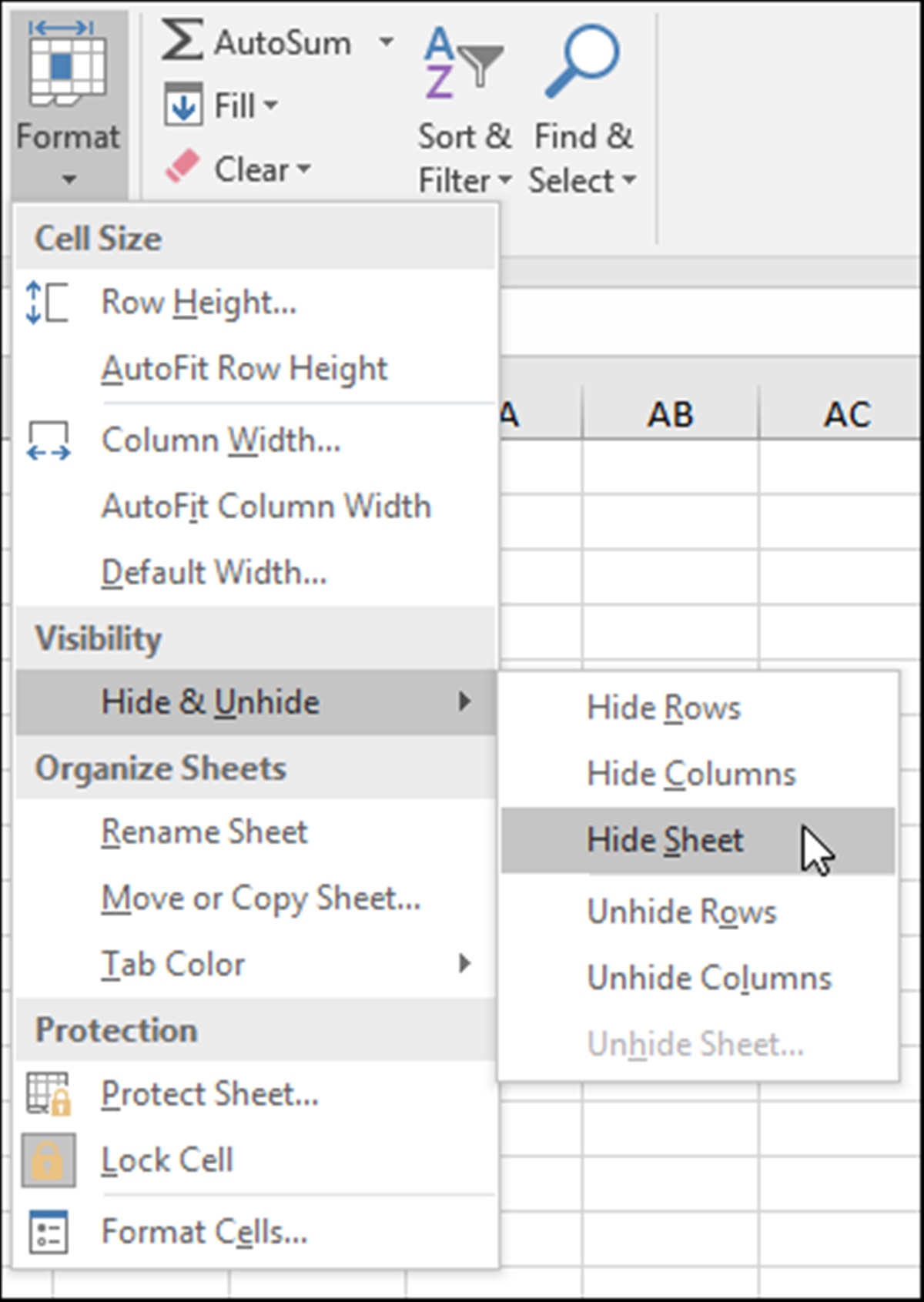
2. Using the Format menu option: Go to the “Home” tab, click on the “Format” dropdown, navigate to the “Visibility” section, and select “Hide Sheet.” This will hide the active worksheet.
3. Using the keyboard shortcut (Ctrl+Shift+0): Press Ctrl+Shift+0 (zero) simultaneously to quickly hide the currently active worksheet.
4. Using the VBA code (Visual Basic for Applications): If you’re familiar with VBA, you can use the following code to hide a worksheet: Sheet1.Visible = False. Replace “Sheet1” with the name of the worksheet you want to hide.
5. Using the Hide Sheet option in the Protect Workbook menu: On the “Review” tab, click on “Protect Workbook” and choose the “Hide Sheet” option. You can then select the worksheet(s) you want to hide and click “OK” to apply the changes.
These methods will help you hide a worksheet in Excel, whether you need to temporarily remove it from view or keep it hidden from other users. Remember, the hidden worksheet can still be accessed and unhidden if needed.
Using the Hide option in the Right-Click menu
One of the easiest ways to hide a worksheet in Excel is by using the hide option in the right-click menu. Follow these simple steps to hide a worksheet:
1. Right-click on the worksheet tab: Locate the tab of the worksheet you want to hide at the bottom of the Excel window. Right-click on the tab to bring up the context menu.
2. Select the Hide option: In the right-click menu, you will see a list of options. Choose the “Hide” option, and the selected worksheet will disappear from view.
3. Verify the hidden worksheet: After selecting the hide option, the hidden worksheet will no longer be visible on the Excel workspace. However, you can still see the hidden worksheet listed among the other sheet tabs.
4. Unhide the worksheet: To unhide the hidden worksheet, right-click on any visible tab, and select “Unhide” from the context menu. You will then see a dialog box displaying all the hidden worksheets. Choose the worksheet you want to unhide and click “OK.”
Using the hide option in the right-click menu is a quick and straightforward method to temporarily remove a worksheet from view. It is especially useful when you want to focus on other worksheets or keep certain data hidden from other users. However, keep in mind that the hidden worksheet can still be accessed and unhidden by following the unhide steps.
Using the Format menu option
Excel provides a convenient Format menu option to hide worksheets. This method allows you to hide a worksheet with just a few clicks. Follow the steps below to use the Format menu option:
1. Go to the “Home” tab: Open the Excel workbook and navigate to the “Home” tab located in the Excel ribbon.
2. Click on the “Format” dropdown: In the “Cells” section of the “Home” tab, you will find the “Format” dropdown menu. Click on it to reveal more formatting options.
3. Select “Visibility” and choose “Hide Sheet”: Within the “Format” dropdown, you will find a section called “Visibility.” Click on it and select the “Hide Sheet” option. This action will hide the active worksheet from view.
4. Verify the hidden worksheet: After selecting “Hide Sheet,” the worksheet you chose will no longer be visible on the Excel workspace. However, it will still be listed among the other sheet tabs.
5. Unhide the worksheet: To unhide the hidden worksheet, follow the process again, but this time select the “Unhide Sheet” option from the “Visibility” section. A dialog box will appear displaying all the hidden worksheets. Choose the worksheet you want to unhide and click “OK.”
The Format menu option in Excel provides a user-friendly way to hide and unhide worksheets. It is a handy method when you need to temporarily conceal a worksheet or keep sensitive information hidden. Remember that the hidden worksheet can be easily unhidden by following the steps mentioned above, so it is not a foolproof method for securing confidential data.
Using the keyboard shortcut (Ctrl + Shift + 0)
An efficient way to hide a worksheet in Excel is by utilizing the keyboard shortcut. Excel provides a specific shortcut, Ctrl + Shift + 0 (zero), to quickly hide the active worksheet. Follow the steps below to use this keyboard shortcut:
1. Select the worksheet to hide: Click on the worksheet tab of the Excel workbook to make it the active sheet.
2. Press the Ctrl + Shift + 0 keys: Simultaneously press the Ctrl, Shift, and number zero (0) keys on your keyboard. This will instantly hide the active worksheet.
3. Verify the hidden worksheet: After using the keyboard shortcut, the hidden worksheet will no longer be visible on the Excel workspace. However, it will still be present in the sheet tabs at the bottom of the window.
4. Unhide the worksheet: To unhide the hidden worksheet, follow the steps mentioned earlier for the specific method you used to hide the worksheet. For example, you can right-click on any visible tab, select “Unhide,” and then choose the sheet you want to unhide from the list.
The keyboard shortcut Ctrl + Shift + 0 provides a quick and convenient way to hide a worksheet without navigating through menus or options. It is especially useful when you need to switch between multiple worksheets or temporarily hide particular data. Remember to use the appropriate method to unhide the worksheet when needed, as the hidden worksheet can be easily revealed using the unhide steps.
Using the VBA code (Visual Basic for Applications)
Excel’s VBA (Visual Basic for Applications) allows for advanced customization and automation within the software. You can use VBA code to hide a worksheet programmatically. Here’s how:
1. Open the Visual Basic Editor: In Excel, press Alt + F11 to open the Visual Basic Editor (VBE). Alternatively, you can go to the “Developer” tab, click on “Visual Basic” in the “Code” group, or use the keyboard shortcut Alt + R + V.
2. Insert a new module: In the VBE, go to “Insert” in the top menu and choose “Module.” This will insert a new module into the project.
3. Write the VBA code: In the module window, write the following code to hide a worksheet:
Sub HideWorksheet()
Sheets(“Sheet1”).Visible = False
End Sub
Replace “Sheet1” with the name of the worksheet you want to hide.
4. Run the code: Close the VBE and return to the Excel worksheet. Press Alt + F8 to open the “Macro” dialog box. Select the “HideWorksheet” macro and click “Run.” The specified worksheet will be hidden.
5. Unhide the worksheet: To unhide the worksheet, you can either modify the VBA code to set the worksheet’s “Visible” property to “xlSheetVisible” or use one of the unhide methods mentioned earlier.
Using VBA code to hide worksheets provides flexibility and automation options for managing your Excel files. It is especially useful when you need to apply specific conditions or trigger hiding actions based on certain events or calculations. However, it requires some familiarity with VBA programming. Remember to save your Excel file in macro-enabled format (.xlsm) to retain the VBA code functionality.
Using the Hide Sheet option in the Protect Workbook menu
Excel provides a built-in feature to protect workbooks and, within that feature, an option to hide worksheets. This method allows you to hide a worksheet while also protecting the workbook. Here’s how to use the Hide Sheet option in the Protect Workbook menu:
1. Go to the “Review” tab: Open the Excel workbook and navigate to the “Review” tab located in the Excel ribbon.
2. Click on “Protect Workbook”: In the “Changes” section of the “Review” tab, you will find the “Protect Workbook” button. Click on it to access the Protect Workbook menu.
3. Select “Hide Sheet”: In the Protect Workbook menu, you will see various options for protecting your workbook. Choose the “Hide Sheet” option to hide the active worksheet.
4. Protect the workbook (optional): If you want to protect the entire workbook from further changes, you can set a password or apply specific protection settings using the options in the Protect Workbook menu.
5. Verify the hidden worksheet: After selecting “Hide Sheet” and potentially protecting the workbook, the worksheet you chose will no longer be visible on the Excel workspace. It will be hidden from view, even if someone tries to unhide it through conventional methods.
6. Unhide the worksheet: To unhide the hidden worksheet, go back to the Protect Workbook menu by clicking on “Protect Workbook” on the “Review” tab. Choose the “Unhide Sheet” option to reveal the hidden worksheet.
Hiding a worksheet using the Hide Sheet option in the Protect Workbook menu provides an added layer of protection for sensitive data. It ensures that the worksheet remains hidden, even if someone tries to unhide it using standard Excel methods. Remember to safeguard and securely store the workbook’s password if you choose to protect the entire workbook.
Methods to Unhide a Worksheet in Excel
After hiding a worksheet in Excel, you may need to unhide it at some point. Excel offers various methods to unhide hidden worksheets, ensuring that you can easily access the data when needed. Here are five different methods to unhide a worksheet in Excel:
1. Using the Unhide option in the Right-Click menu: Right-click on any visible worksheet tab, and select “Unhide” from the context menu. A dialog box will appear showing a list of hidden worksheets. Choose the worksheet you want to unhide and click “OK.”
2. Using the Format menu option: Go to the “Home” tab, click on the “Format” dropdown in the “Cells” section, and select “Unhide Sheet.” This will display a dialog box listing the hidden worksheets. Choose the worksheet you want to unhide and click “OK.”
3. Using the keyboard shortcut (Ctrl + Shift + 9): Press Ctrl + Shift + 9 simultaneously to quickly unhide the first hidden worksheet in the workbook. If there are multiple hidden worksheets, you can repeat the shortcut to unhide the next one, and so on.
4. Using the VBA code (Visual Basic for Applications): If you hid the worksheet using VBA code, you can use VBA again to unhide it. Open the Visual Basic Editor, locate the module with the hiding code, and modify it to set the worksheet’s “Visible” property to “xlSheetVisible”.
5. Using the Unhide Sheet option in the Protect Workbook menu: On the “Review” tab, click on “Protect Workbook” and choose the “Unhide Sheet” option. A dialog box will appear showing the hidden worksheets. Select the worksheet you want to unhide and click “OK.”
By using these methods, you can easily unhide a worksheet in Excel, whether you intentionally hid it or need to access hidden data. Remember to use the appropriate method based on how the worksheet was hidden, and ensure that you have the necessary permissions or password to unhide protected sheets.
Using the Unhide option in the Right-Click menu
If you have hidden a worksheet in Excel and need to make it visible again, one of the easiest methods to unhide a worksheet is by using the unhide option in the right-click menu. Follow these simple steps:
1. Right-click on any visible worksheet tab: Find any visible worksheet tab located at the bottom of the Excel window. Right-click on the tab to open the context menu.
2. Select the Unhide option: In the right-click menu, you will see a list of options. Choose the “Unhide” option, and a dialog box will appear, displaying a list of hidden worksheets.
3. Select the worksheet to unhide: From the list of hidden worksheets, choose the one you want to make visible again. Click on it to highlight the sheet and click “OK.”
4. Verify the unhidden worksheet: After clicking “OK,” the previously hidden worksheet will become visible and reappear on the Excel workspace. You can now access and work with the unhidden worksheet.
The unhide option in the right-click menu provides a quick and straightforward way to make hidden worksheets visible again. This method is especially useful when you have hidden multiple sheets and need to selectively unhide specific ones. Remember that hidden worksheets will remain hidden until you manually unhide them using this method or another unhide technique.
Using the Format menu option
Excel’s Format menu provides a convenient method to unhide hidden worksheets and make them visible again. Here’s how to use the Format menu option to unhide a worksheet:
1. Go to the “Home” tab: Open the Excel workbook and navigate to the “Home” tab located in the Excel ribbon.
2. Click on the “Format” dropdown: In the “Cells” section of the “Home” tab, you will find the “Format” dropdown menu. Click on it to reveal more formatting options.
3. Select “Unhide Sheet”: Within the “Format” dropdown, locate the “Visibility” section and select the “Unhide Sheet” option. This action will display a dialog box listing any hidden worksheets.
4. Select the worksheet to unhide: In the “Unhide Sheet” dialog box, you will see a list of hidden worksheets. Choose the worksheet you want to unhide by clicking on it, and then click “OK.”
5. Verify the unhidden worksheet: After clicking “OK,” the hidden worksheet will become visible again and reappear on the Excel workspace. You can now access and work with the unhidden worksheet.
The Format menu option provides a user-friendly and easily accessible way to unhide hidden worksheets in Excel. It is particularly useful when you have hidden multiple sheets and need to selectively unhide specific ones. Remember that hidden worksheets will remain hidden until you manually unhide them using this method or another unhide technique.
Using the keyboard shortcut (Ctrl + Shift + 9)
Unhiding a hidden worksheet in Excel can be done quickly and conveniently using a keyboard shortcut. Excel provides a specific shortcut, Ctrl + Shift + 9, to unhide the first hidden worksheet in the workbook. Here’s how to use this shortcut:
1. Select a visible worksheet: Ensure that you have any visible worksheet selected in Excel.
2. Press the Ctrl + Shift + 9 keys: Simultaneously press the Ctrl, Shift, and number nine (9) keys on your keyboard. This will instantly unhide the first hidden worksheet in the workbook.
3. Verify the unhidden worksheet: After using the keyboard shortcut, the previously hidden worksheet will become visible again and reappear on the Excel workspace. You can now access and work with the unhidden worksheet.
4. Repeat the shortcut (if needed): If you have multiple hidden worksheets and want to unhide them one by one, you can repeat the Ctrl + Shift + 9 shortcut to unhide additional hidden sheets.
Using the keyboard shortcut Ctrl + Shift + 9 provides a quick and efficient way to unhide the first hidden worksheet in Excel. It is especially handy when you have only one hidden sheet and need to make it visible again without navigating through menus or options. However, please note that this shortcut unhides only the first hidden worksheet, so if you have multiple hidden sheets, you will need to repeat the shortcut to unhide the rest.
Using the VBA code (Visual Basic for Applications)
Unhiding a hidden worksheet in Excel can be accomplished using VBA (Visual Basic for Applications) code. VBA allows for automation and customization of Excel, including unhiding hidden sheets. Here’s how to use VBA code to unhide a worksheet:
1. Open the Visual Basic Editor: In Excel, press Alt + F11 to open the Visual Basic Editor (VBE). Alternatively, you can go to the “Developer” tab, click on “Visual Basic” in the “Code” group, or use the keyboard shortcut Alt + R + V.
2. Locate the VBA code: In the VBE, locate the VBA code responsible for hiding the worksheet. This code may exist within a module, a worksheet object, or the ThisWorkbook object.
3. Modify the code: Depending on how the worksheet was hidden, modify the VBA code to unhide the worksheet. For example, if the code used the “Visible” property and set it to “False” to hide the worksheet, change it to “True” to unhide the sheet.
4. Run the code: Close the VBE and return to the Excel workbook. Press Alt + F8 to open the “Macro” dialog box. Select the macro that contains the modified code to unhide the worksheet and click “Run.” The hidden worksheet will become visible again.
Using VBA code to unhide a worksheet in Excel allows for automation and customization, especially when you need to unhide sheets based on specific conditions or events. It provides flexibility and control over unhiding operations. Remember to save your Excel file in the macro-enabled format (.xlsm) to retain the functionality of the VBA code.
Using the Unhide Sheet option in the Protect Workbook menu
When a worksheet is hidden within a protected workbook, you can use the “Unhide Sheet” option in the Protect Workbook menu to make it visible again. Here’s how to unhide a hidden worksheet using this method:
1. Go to the “Review” tab: Open the Excel workbook and navigate to the “Review” tab located in the Excel ribbon.
2. Click on “Protect Workbook”: In the “Changes” section of the “Review” tab, you will find the “Protect Workbook” button. Click on it to access the Protect Workbook menu.
3. Select “Unhide Sheet”: In the Protect Workbook menu, you will see various options for protecting your workbook. Choose the “Unhide Sheet” option. A dialog box will appear, displaying a list of hidden worksheets.
4. Select the worksheet to unhide: From the list of hidden worksheets in the dialog box, choose the worksheet you want to make visible again. Click on it to select it and then click “OK.”
5. Verify the unhidden worksheet: After clicking “OK,” the previously hidden worksheet will become visible again and reappear on the Excel workspace. You can now access and work with the unhidden worksheet.
By using the Unhide Sheet option in the Protect Workbook menu, you can easily unhide a hidden worksheet within a protected workbook. This method ensures that the worksheet remains hidden from view until specifically unhidden using the Protect Workbook menu. However, keep in mind that the effectiveness of this method relies on the protection applied to the workbook.
Tips and Tricks for Hiding and Unhiding Worksheets
Hiding and unhiding worksheets in Excel can be incredibly useful for organizing data and managing workbooks. Here are some tips and tricks to enhance your experience when hiding and unhiding worksheets:
1. Hiding multiple worksheets simultaneously: To hide multiple worksheets at once, press and hold the Ctrl key, select the tabs of the worksheets you want to hide, right-click on any selected tab, and choose the “Hide” option from the context menu. This allows for faster and more efficient hiding of multiple sheets.
2. Creating a custom shortcut key for hiding/unhiding worksheets: Excel provides the option to assign custom shortcut keys for various commands. You can assign your own shortcut key combination to the Hide or Unhide Sheet commands to make the process even quicker. To do this, go to “File” > “Options” > “Customize Ribbon” > “Customize” > “Keyboard Shortcuts.” Then, choose the appropriate command and specify your desired shortcut key combination.
3. Protecting hidden worksheets: By default, hidden worksheets can still be accessed and even modified by anyone with access to the workbook. To protect hidden worksheets from being unhidden or modified, you can use the Protect Sheet or Protect Workbook features. This adds an extra layer of security to your hidden data.
4. Using named ranges: If you frequently work with hidden worksheets or reference data from hidden worksheets, using named ranges can simplify your formulas and calculations. By assigning a name to a specific range of cells on a hidden worksheet, you can refer to it in formulas without needing to unhide the sheet. This allows you to keep your worksheets hidden while still accessing the necessary data.
5. Adding a color or icon to hidden tabs: To easily identify hidden worksheets, you can apply a unique color or add an icon to their corresponding tabs. This visual cue helps distinguish hidden worksheets from visible ones, making it easier to locate and manage them within large workbooks.
By utilizing these tips and tricks, you can streamline your workflow and effectively hide and unhide worksheets in Excel. Whether it’s hiding multiple sheets at once, assigning custom shortcut keys, protecting hidden data, or simplifying formulas using named ranges, these techniques will enhance your efficiency and organization in Excel.
Hiding multiple worksheets simultaneously
Hiding multiple worksheets in Excel is a common requirement, especially when you want to remove several sheets from view at once. Rather than hiding each sheet individually, Excel provides a convenient way to hide multiple worksheets simultaneously. Here’s how you can achieve this:
1. Press and hold the Ctrl key: To select multiple worksheets, press and hold the Ctrl key on your keyboard.
2. Select the tabs of the worksheets to hide: While holding the Ctrl key, click on the sheet tabs of the worksheets you want to hide. Each clicked tab will be selected.
3. Right-click on any selected tab: Once you have selected all the desired worksheets, right-click on any of the selected tabs to bring up the context menu.
4. Choose the “Hide” option: In the right-click menu, select the “Hide” option. This action will hide all the selected worksheets simultaneously.
5. Verify the hidden worksheets: After selecting the “Hide” option, the selected worksheets will no longer be visible on the Excel workspace. However, they will still be listed among the other sheet tabs.
By using this method, you can quickly hide multiple worksheets at once, saving valuable time and effort. It is particularly useful when you need to hide several related sheets or group worksheets for better organization. Remember that hidden worksheets can still be accessed and unhidden using appropriate methods when needed.
Creating a custom shortcut key for hiding/unhiding worksheets
To further streamline your workflow in Excel, you can create custom shortcut keys specifically for hiding and unhiding worksheets. By assigning your own shortcut key combinations, you can quickly toggle the visibility of worksheets with ease. Here’s how you can create custom shortcut keys:
1. Go to “File” > “Options”: Open the Excel workbook and navigate to the “File” tab in the ribbon. Click on “Options” to access the Excel Options dialog box.
2. Select “Customize Ribbon” > “Customize”: In the Excel Options dialog box, choose “Customize Ribbon” from the left sidebar. Then, click on the “Customize” button next to the “Keyboard shortcuts” option at the bottom.
3. Choose the appropriate category and command: In the Customize Keyboard dialog box, select the appropriate category from the “Categories” list. For example, to assign a shortcut for hiding worksheets, you might select the “All Commands” category.
4. Locate and select the command: After selecting the category, scroll down the “Commands” list to find the specific command you want to assign a shortcut to. For example, choose “HideSheet” for hiding worksheets.
5. Specify your desired shortcut key combination: In the “Press new shortcut key” field, press the keys you want to use for your custom shortcut. Make sure the combination is not already assigned to another command. Excel will notify you if the shortcut is already in use.
6. Click “Assign” and then “Close”: Once you’ve entered your desired shortcut key combination, click “Assign” to assign it to the selected command. Afterward, click “Close” to exit the Customize Keyboard dialog box.
By creating custom shortcut keys, you can hide and unhide worksheets in Excel by simply pressing your chosen key combination. This saves time and eliminates the need to navigate menus or use default shortcuts. Remember to choose unique and memorable key combinations while avoiding conflicts with existing shortcuts.
Protecting hidden worksheets
When working with hidden worksheets in Excel, you may want to ensure that the hidden data remains protected from accidental or unauthorized access. Excel provides built-in protection features that allow you to not only hide worksheets but also protect them from being unhidden or modified. Here’s how you can protect hidden worksheets in Excel:
1. Hide the worksheet: Before protecting a hidden worksheet, make sure you have hidden the worksheet using one of the available methods mentioned earlier.
2. Go to the “Review” tab: Open the Excel workbook and navigate to the “Review” tab located in the Excel ribbon.
3. Click on “Protect Workbook”: In the “Changes” section of the “Review” tab, you will find the “Protect Workbook” button. Click on it to access the Protect Workbook menu.
4. Select the desired protection options: In the Protect Workbook menu, you will find various protection options. Configure the settings according to your requirements. You may choose to set a password, specify protection options like prohibiting worksheet deletion or modification, or both.
5. Apply the protection: Once you have selected the desired protection options, click on “OK” to apply the protection to the workbook.
Now, the hidden worksheets within your protected workbook are not only hidden but also safeguarded by the applied protection. This adds an extra layer of security, ensuring that the hidden data remains inaccessible and unmodifiable. Even if someone tries to unhide the worksheets using conventional methods, they won’t be able to do so unless they have the necessary password or permission to modify the protected workbook.
Protecting hidden worksheets is particularly useful when dealing with confidential or sensitive data that you want to keep hidden from unauthorized individuals. However, it’s important to remember to store the password securely if you have chosen to set one, as losing or forgetting the password can lead to permanent data loss or difficulties in accessing the hidden information.