How to Group in Excel

What is Grouping in Excel?

Grouping in Excel is a powerful feature that allows you to organize and manipulate data by consolidating related rows or columns together. It helps you effectively manage large sets of information, making it easier to analyze and present your data in a more structured and digestible format.

When you group data in Excel, you can collapse or expand the grouped sections to hide or display specific details. This can be particularly useful when dealing with extensive datasets or when you want to focus on specific subsets of information without getting overwhelmed by all the data at once.

With Excel’s grouping feature, you can group both rows and columns based on various criteria, including numeric values, text, dates, or custom formulas. This flexibility allows you to tailor the grouping to suit your specific data organization needs.

By grouping rows and columns, you can create a hierarchical structure within your data, making it easier to navigate and analyze. This can be particularly beneficial when dealing with complex datasets or when preparing reports that require a clear presentation of information.

Grouping in Excel also offers a range of additional functionalities, such as adding summary information, performing calculations on grouped data, and even grouping data in PivotTables for more advanced data analysis.

Overall, the grouping feature in Excel provides a powerful tool for organizing and manipulating data, enabling you to work more efficiently and effectively with large datasets. Whether you need to analyze financial data, manage project timelines, or track sales figures, mastering the grouping feature in Excel can significantly enhance your productivity and data management capabilities.

How to Group Rows and Columns in Excel

Grouping rows and columns in Excel is a straightforward process that can greatly help in organizing and managing your data. There are two primary methods to achieve this – using the Group feature and using the Outline feature. Let’s explore each method in detail:

Grouping Rows and Columns Using the Group Feature

To group rows or columns using the Group feature:

Select the range of rows or columns that you want to group.
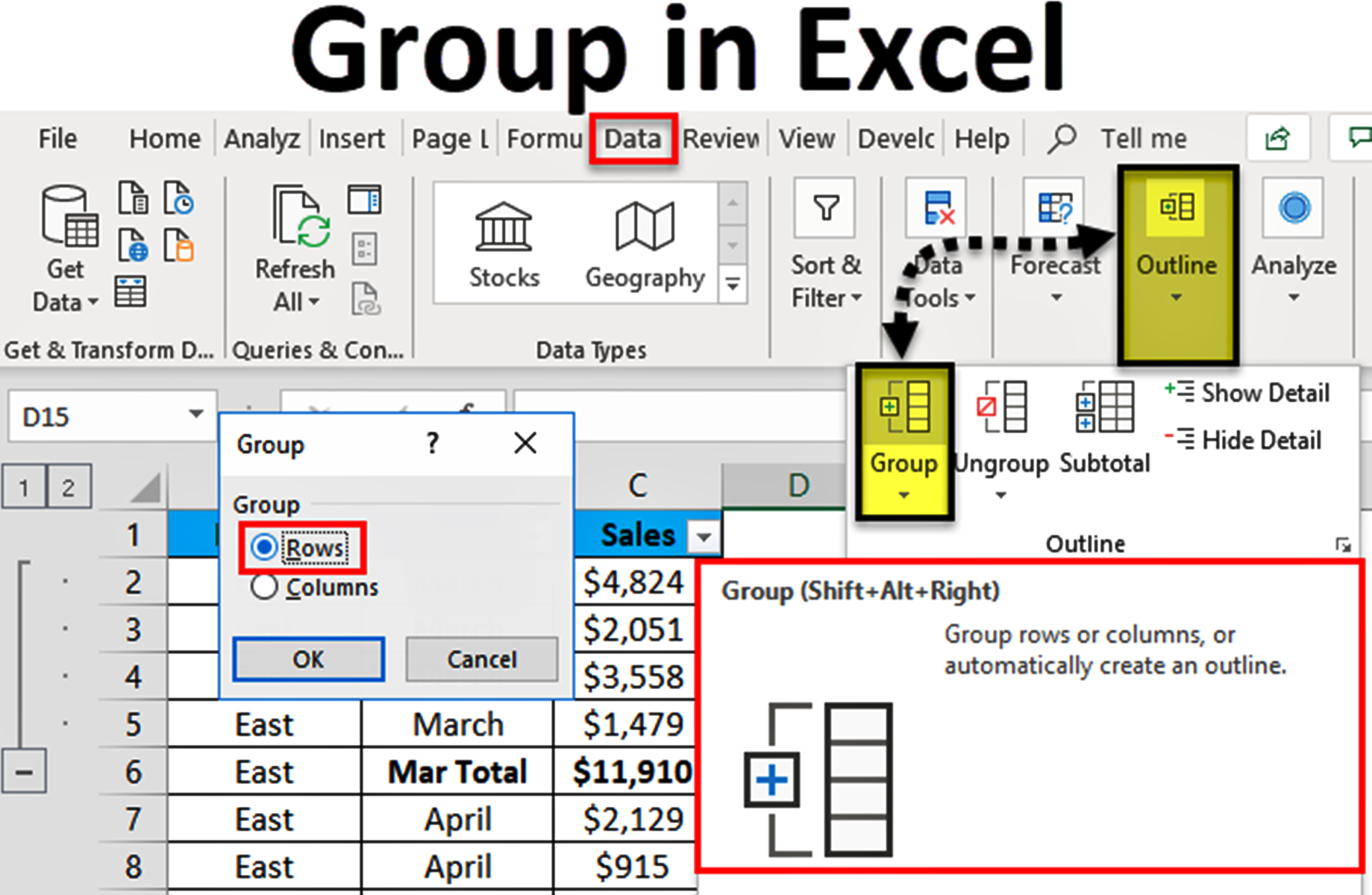
Right-click on the selected range and choose “Group” from the context menu, or go to the “Data” tab in the ribbon and click on the “Group” button.
You will notice that Excel adds a small symbol (either a “-” or “+”) next to the row or column that represents the grouped range.
To collapse or expand the grouped range, simply click on the symbol. This allows you to easily hide or show the grouped data as needed.

Grouping Rows and Columns Using the Outline Feature

The Outline feature offers a more comprehensive way to group data in Excel:

Select the range of rows or columns that you want to group.
Go to the “Data” tab in the ribbon and click on the “Group” button.
Excel will display an outline panel on the left side of the screen, allowing you to expand or collapse the grouped sections.
Clicking on the “+” or “-” symbols in the outline panel lets you expand or collapse the groups, respectively.

With both methods, you can easily group multiple rows or columns together based on specific criteria, such as dates, values, or text. This can significantly enhance data organization and simplify the analysis and presentation of information.

Remember that you can always adjust the grouping by adding or removing rows or columns from the existing group. Additionally, Excel provides options to hide or display the outlining symbols for a cleaner look.

Learning to group rows and columns in Excel is a valuable skill that can save you time and improve the way you work with data. Whether you are managing complex spreadsheets, creating reports, or performing data analysis, using the grouping feature can make your tasks more efficient and streamlined.

Grouping Rows and Columns Using the Group Feature

Grouping rows and columns in Excel using the Group feature is a simple and effective way to organize and manage your data. This feature allows you to collapse or expand groups of rows or columns, providing a cleaner and more organized view of your data. Here’s how you can use the Group feature in Excel:

Select the range of rows or columns that you want to group. This can be done by clicking and dragging your mouse over the desired range.
Right-click on the selected range and choose the “Group” option from the context menu. Alternatively, you can navigate to the “Data” tab in the ribbon and click on the “Group” button.
Excel will automatically add a small symbol, either a “-” or “+”, next to the row number or column letter that represents the grouped range.
To collapse or expand the grouped range, simply click on the symbol. This allows you to hide or show the grouped data as needed.

The Group feature is particularly useful when dealing with large datasets or when you want to focus on specific sections of your data. For example, if you have a spreadsheet with sales data for multiple regions, you can group the rows corresponding to each region. This way, you can easily collapse the groups for regions that are not currently of interest, and expand them when needed.

You can also create multiple levels of grouping by selecting different ranges and applying the Group feature. This allows you to create a hierarchical structure for your data, making it even easier to navigate and analyze.

It’s important to note that when you group rows or columns, Excel automatically adds an outline to the left and above the grouped range. This outline allows you to collapse or expand groups at a higher level, rather than individually collapsing or expanding each group.

To adjust the grouping or remove it altogether, you can right-click on the grouped symbol and choose the “Ungroup” option from the context menu. Excel also provides options to customize the appearance of the grouping symbols to suit your preferences.

By utilizing the Group feature in Excel, you can effectively organize and manage your data, improving both the efficiency and clarity of your spreadsheets. Whether you are working with financial data, project timelines, or any other type of information, grouping rows and columns can simplify your analysis and enhance your overall productivity.

Grouping Rows and Columns Using the Outline Feature

In addition to the Group feature, Excel offers the Outline feature, which provides a more comprehensive way to group rows and columns. The Outline feature allows you to create a hierarchical structure within your data, making it easier to navigate and analyze. Here’s how you can use the Outline feature to group rows and columns in Excel:

Select the range of rows or columns that you want to group. This can be done by clicking and dragging your mouse over the desired range.
Navigate to the “Data” tab in the ribbon and click on the “Group” button. Excel will display an outline panel on the left side of the screen.
Click on the “+” symbol in the outline panel to expand the grouped sections or click on the “-” symbol to collapse them.

The Outline feature offers a more visual and intuitive way to manage grouped data. It provides a clear overview of the hierarchy and allows you to expand or collapse multiple groups at once.

With the Outline feature, you can create multiple levels of grouping by selecting different ranges and applying the Group function. This enables you to create a nested structure for your data, providing a more detailed organization.

One advantage of using the Outline feature is the capability to display summary information for each group. Excel automatically inserts a summary row or column for each group, which can include functions such as sum or average. This summary information allows you to quickly analyze the data within each group without manually performing calculations.

Additionally, the Outline feature offers various customization options. You can adjust the level of detail shown in the outline by collapsing or expanding levels individually or all at once. It is also possible to show or hide the outline symbols to declutter the view of your spreadsheet.

The Outline feature is especially useful when working with extensive datasets or when you need a clear and comprehensive view of your grouped data. It streamlines the process of accessing and analyzing information within the groups, making it easier to identify patterns and trends.

To remove the outline and ungroup rows or columns, you can navigate to the “Data” tab, click on the “Ungroup” button, and follow the instructions.

By leveraging the power of the Outline feature in Excel, you can effectively organize and manage your data, enhancing both the efficiency and readability of your spreadsheets. Whether you are dealing with project plans, sales data, or any other type of information, grouping rows and columns using the Outline feature provides a valuable tool for data organization and analysis.

Expanding and Collapsing Groups in Excel

When you group rows or columns in Excel, you gain the ability to expand or collapse these groups, allowing you to control the level of detail displayed in your spreadsheet. This feature is incredibly useful when working with large datasets or when you want to focus on specific sections of your data. Here’s how you can expand and collapse groups in Excel:

Expanding Groups:

Locate the grouped symbol, which is typically a “+” symbol, next to the row number or column letter that represents the grouped range.
Click on the “+” symbol to expand the associated group.
All the rows or columns contained within the group will now be visible, displaying the detailed data.

Collapsing Groups:

Locate the grouped symbol, which is typically a “-” symbol, next to the row number or column letter that represents the grouped range.
Click on the “-” symbol to collapse the associated group.
The detailed data within the group will no longer be visible, providing a more summarized view of the data.

By expanding and collapsing groups, you can navigate through large datasets with greater ease and focus on the specific information you need. This functionality allows you to hide irrelevant or detailed data temporarily, reducing visual clutter and improving overall readability.

It’s important to note that you can expand or collapse individual groups or work with multiple groups simultaneously. Excel’s grouping feature allows you to expand or collapse all groups at once, making it convenient for managing large sets of data.

In addition to expanding or collapsing groups at the individual level, you can also expand or collapse groups at higher levels using the outline symbols. These symbols appear on the left side of the spreadsheet when you apply grouping in Excel. By clicking on the corresponding symbols, you can expand or collapse groups across different sections of your data, providing a more comprehensive control over the level of detail displayed.

Expanding and collapsing groups in Excel is a powerful tool that helps you easily manage and analyze your data. Whether you’re presenting information to others or performing in-depth data analysis, this feature allows you to strike the right balance between providing necessary details and maintaining a concise view of your spreadsheet.

Adding Summary Information with Grouping in Excel

One of the key benefits of grouping in Excel is the ability to automatically add summary information for each group. This feature allows you to obtain aggregated data, such as totals or averages, without the need for manual calculations. Here’s how you can add summary information with grouping in Excel:

Select the range of rows or columns that you want to group.
Apply the grouping feature using either the Group or Outline method, as previously discussed.
Excel will automatically insert a summary row or column for each group, placed at the end of the group.
Using the functions available in Excel, such as sum, average, count, or custom formulas, you can calculate the desired summary information for each group.

By adding summary information, you can quickly analyze and compare data within each group, providing valuable insights in a concise format. This functionality is particularly useful when working with large datasets or when you need to present summarized data in reports or presentations.

Excel offers a wide range of built-in functions that you can use to calculate summary information. For example, you can use the SUM function to add up values, the AVERAGE function to determine the average value, or the COUNT function to count the number of entries within a group. Additionally, you can create custom formulas that meet specific requirements.

Once you have added the summary formulas, Excel will update the summary information automatically whenever you modify the values within the grouped range. This ensures that the summary data remains accurate and up to date.

To make the summary information more visually appealing and distinguishable, you can apply formatting options, such as bold or italic text, color coding, or border styles.

Furthermore, Excel provides options to customize the appearance of the summary rows or columns. You can choose to show or hide the summary rows or columns, depending on your preference. This flexibility allows you to adjust the level of detail displayed in your spreadsheet, catering to your specific data presentation needs.

By using the grouping feature in Excel and incorporating summary information, you can streamline your analysis process and make informed decisions. Whether you’re analyzing sales data, managing project timelines, or tracking expenses, the ability to easily calculate and view summary information by group can greatly enhance your data organization and understanding.

Grouping Data in Pivot Tables

Pivot tables are a powerful feature in Excel that allow you to analyze and summarize large amounts of data. They provide a flexible and dynamic way to group and categorize data, making it easier to understand and draw insights. Here’s how you can group data in pivot tables:

Create a pivot table by selecting the data range and choosing “PivotTable” from the “Insert” tab in the ribbon.
In the pivot table field list, drag the desired field(s) to the “Rows” or “Columns” area.
Right-click on a value in the pivot table and select “Group” from the context menu.
Specify the grouping criteria, such as date intervals, numeric ranges, or custom categories.
Click “OK” to group the data in the pivot table.

By grouping data in pivot tables, you can arrange and summarize your data in a meaningful way. This can be particularly useful when working with time-based data, allowing you to group dates by months, quarters, or years. For numerical data, grouping can help analyze data in specific ranges, such as grouping sales amounts into different revenue brackets.

Pivot tables also offer options to customize the grouping, such as adding subtotals and grand totals, as well as sorting the groups in ascending or descending order. This allows you to tailor the presentation of your data to meet your analysis needs.

One advantage of grouping data in pivot tables is the ability to easily expand or collapse the groups to focus on specific subsets of data. This provides a dynamic and interactive way to explore and analyze different levels of detail without modifying or rearranging the original data.

In addition to grouping data in rows or columns, you can also apply grouping to the values in a pivot table. This enables you to categorize and summarize numerical data based on specific criteria, such as grouping sales by product categories or grouping expenses by departments.

By grouping data in pivot tables, you can gain deeper insights and uncover patterns and trends within your data. This feature is particularly valuable for data analysis, reporting, and decision-making, allowing you to effectively summarize and present complex information in a structured manner.

Remember that you can always modify or remove the grouping in a pivot table to adapt to changing analysis requirements. Simply right-click on a grouped value in the pivot table, select “Ungroup,” and make the necessary adjustments.

Utilizing the grouping feature in pivot tables expands the capabilities of Excel, enabling you to efficiently analyze and present data. Whether you’re conducting financial analyses, performing sales analysis, or examining any other type of dataset, grouping data in pivot tables provides a powerful tool for dynamic data exploration and visualization.

Grouping Dates in Excel

When working with date data in Excel, grouping dates can provide a clearer and more organized view of your data. Grouping dates allows you to categorize and summarize your data by specific time periods, making it easier to analyze trends and patterns. Here’s how you can group dates in Excel:

Select the range of cells containing the date data that you want to group.
Right-click on the selected range and choose “Group” from the context menu.
Excel will display a dialog box that allows you to select the period of time by which you want to group the dates, such as months, years, quarters, or any other custom interval.
Select the desired time period and click “OK”.

By grouping dates, Excel will automatically create expandable and collapsible groups based on the specified time period. This allows you to easily hide or show details for a specific time period, improving the readability and manageability of your data.

The grouping feature also enables you to add additional summary information to each date group. For example, you can use built-in functions like SUM, AVERAGE, COUNT, or MAX to calculate total sales, average daily revenue, or the highest value within each group.

When grouping dates, it’s important to ensure that Excel recognizes your data as dates. This is especially crucial if your dates are entered as text or in a non-standard format. To convert your text or non-standard dates into Excel’s date format, select the range of cells, go to the “Number Format” drop-down in the ribbon, and choose the desired date format.

Excel also provides options to customize the appearance of the grouped dates. You can choose to display the groupings as specific formats, such as “January 2022,” or use a more compact format like “Jan-22”. You can modify the formatting by right-clicking on the grouped dates, selecting “Group Field Settings,” and adjusting the format settings.

Grouping dates in Excel is extremely useful when analyzing time-based data. For instance, you can group sales data by month to identify seasonal trends, or group expenses by quarter for better financial planning. It allows you to condense and summarize large amounts of data into manageable units, providing a clearer view of your analysis.

Remember that you can always modify or remove the grouping if needed. Simply right-click on a grouped date range, choose “Ungroup,” and make the necessary adjustments.

Grouping dates in Excel is a valuable technique for organizing and analyzing time-based data. By utilizing this feature, you can easily navigate and interpret your data, uncover insights, and make informed decisions.

Grouping Numbers in Excel

Grouping numbers in Excel is a powerful feature that allows you to organize and summarize numerical data. By grouping numbers, you can create categories or ranges to simplify analysis and enhance data visualization. Here’s how you can group numbers in Excel:

Select the range of cells containing the numerical data that you want to group.
Right-click on the selected range and choose “Group” from the context menu.
Excel will display a dialog box that allows you to specify the group intervals or ranges.
Enter the desired values for the start and end points of each group, or choose the interval size if you want equal-sized groups.
Click “OK” to apply the grouping to your numerical data.

By grouping numbers in Excel, you can condense your data into meaningful categories or ranges. This can be particularly useful when working with numerical data such as sales figures, product prices, or age ranges. Grouping numbers allows you to analyze trends, identify outliers, and gain a better understanding of your data.

Excel also provides options to customize the appearance of the grouped numbers. You can modify the format of the group labels, such as showing a range like “0-100,” or use custom labels to describe the groupings in a more meaningful way.

When you group numbers, Excel automatically adds outlining symbols to the left of the grouped range. This allows you to expand or collapse the groups, providing a more focused view of your data. You can use the “+” and “-” symbols to expand or collapse individual groups or utilize the outline symbols to expand or collapse groups at higher levels.

Furthermore, you can add summary information to your grouped numerical data using functions such as SUM, AVERAGE, COUNT, or any other relevant calculation. This enables you to obtain meaningful insights and perform quick analyses on your categorized data.

It’s important to keep in mind that when working with very large datasets, grouping numbers may impact the performance of your Excel workbook. In such cases, consider using other methods, such as creating a pivot table or employing formulas, to summarize and analyze your data.

To modify or remove the grouping of numbers, you can right-click on a grouped range, choose “Ungroup,” and make the necessary adjustments.

Grouping numbers in Excel is a valuable technique for simplifying data analysis and visualization. By categorizing numerical data, you can identify patterns, highlight key information, and gain deeper insights into your dataset.

Grouping Text in Excel

Grouping text in Excel allows you to categorize and organize textual data to simplify analysis and improve data management. By grouping text, you can create logical groupings, such as categories or subcategories, that make it easier to explore and understand your data. Here’s how you can group text in Excel:

Select the range of cells containing the text data that you want to group.
Right-click on the selected range and choose “Group” from the context menu.
Excel will display a dialog box that allows you to specify the criteria for grouping the text.
Enter the desired values or keywords to define the groups, or choose a specific condition based on your text data.
Click “OK” to apply the grouping to your text data.

By grouping text in Excel, you can effectively organize and summarize large amounts of data. This can be particularly useful when working with text data such as product categories, customer segments, or project phases. Grouping text allows you to quickly identify patterns, compare data within and across groups, and gain insights into your dataset.

When grouping text, it’s important to ensure that your text data is consistent and properly formatted. Excel uses the exact text values or specified criteria to group the text, so any inconsistencies or variations may affect the grouping results. You may need to clean and standardize your text data before grouping to ensure accurate groupings.

Excel offers options to customize the appearance of the grouped text. You can modify the format of the group labels to make them more descriptive or visually distinguishable. Additionally, you can add summary information to your grouped text data, such as counts or percentages, to provide additional context or insights.

Excel also provides built-in functions such as COUNTIF, SUMIF, or AVERAGEIF, which can be used to calculate summary information based on the groupings. These functions allow you to analyze and aggregate data within each group, providing valuable information for decision-making and analysis.

To modify or remove text grouping in Excel, you can right-click on a grouped range, choose “Ungroup,” and make the necessary adjustments. This allows you to refine or restructure your groupings as needed.

Grouping text in Excel is a powerful technique for organizing and analyzing textual data. By categorizing and summarizing your text data, you can gain valuable insights, streamline data analysis, and make informed decisions based on the grouped information.

Ungrouping Rows and Columns in Excel

Ungrouping rows and columns in Excel is a simple process that allows you to remove the grouping applied to your data. Whether you want to modify the groupings or analyze the individual data points, ungrouping provides you with the flexibility to work with your data at a granular level. Here’s how you can ungroup rows and columns in Excel:

Ungrouping Rows:

Select the rows that are currently grouped.
Right-click on the selection and choose the “Ungroup” option from the context menu.

Ungrouping Columns:

Select the columns that are currently grouped.
Right-click on the selection and choose the “Ungroup” option from the context menu.

When you ungroup rows or columns, Excel removes the outlining symbols and restores the individual rows or columns to their original state. This allows you to work with the data in its ungrouped form, making it easier to perform specific calculations, apply formatting, or make adjustments as needed.

It’s important to note that ungrouping rows or columns does not remove any additional formatting or calculations applied to your data. It only removes the grouping itself.

When ungrouping data, you can choose to ungroup individual groupings or remove all groupings at once. If you have multiple groups present, you can select multiple grouped ranges and apply the ungrouping action simultaneously.

Ungrouping rows or columns in Excel is useful when you need to work with specific subsets of data or modify the structure of your worksheet. Whether you want to perform detailed calculations, apply conditional formatting, or reorganize your data, ungrouping allows you to regain control and flexibility over your data.

Remember that ungrouping rows or columns does not delete or modify your data in any way. It simply removes the grouping function, allowing you to view and manipulate the data in its individual state.

To adjust or modify groupings, you can reapply the grouping feature to your desired range or make changes to the existing grouping settings.

Ungrouping rows and columns in Excel provides you with the freedom to work with your data in a more customized and detailed manner. By ungrouping, you can navigate and analyze individual data points or make modifications as required for your specific data analysis needs.

Tips and Tricks for Efficient Grouping in Excel

Efficient grouping in Excel can greatly improve your data management and analysis capabilities. By employing some useful tips and tricks, you can make the most of Excel’s grouping feature and streamline your workflow. Here are some tips to help you effectively use grouping in Excel:

Plan your groupings: Before applying groupings, carefully consider the structure and organization of your data. Plan out the desired groups and hierarchies to ensure that the groupings accurately represent your data and support your analysis goals.
Apply consistent formatting: To maintain consistency and make your groupings visually coherent, apply consistent formatting to your grouped rows or columns. This will help you easily identify and navigate through the grouped sections of your data.
Use custom groupings: Excel allows you to create custom groupings based on specific criteria or conditions. Explore the options available to group your data in a way that best suits your analysis needs. For example, you can group data based on a custom formula or use different interval sizes.
Combine grouping methods: Depending on the complexity of your data, you can combine different grouping methods within a worksheet. Use both row and column grouping to create a more comprehensive and detailed hierarchical structure in your data.
Add summary calculations: Take advantage of Excel’s powerful functions to add summary calculations within your grouped sections. Functions like SUM, AVERAGE, COUNT, or MAX can provide instant insights into your data and enhance your analysis.
Utilize expand/collapse shortcuts: Excel offers keyboard shortcuts that allow you to quickly expand or collapse grouped sections. For example, use the “+” or “-” keys on your keyboard to expand or collapse a selected group without the need for right-clicking or navigating through menus.
Reorder groups: Excel allows you to rearrange the order of your grouped sections. This can be helpful if you want to prioritize or rearrange the importance of specific groups within your data hierarchy. Simply click and drag the grouped section to the desired position.
Add group labels: To improve the clarity and understanding of your groupings, consider adding labels to your grouped sections. This can be done by inserting descriptive text or utilizing Excel’s specialized chart elements, such as data labels or trendlines.
Document the groupings: Keep track of your groupings by providing clear documentation or labeling within your spreadsheet. Use comments, annotations, or separate documentation sheets to outline the purpose and criteria of each grouping, making it easier to maintain and update your Excel workbook in the future.
Regularly review and adjust groupings: As your data evolves or analysis requirements change, it’s important to regularly review and adjust your groupings. Periodically assess whether your groupings are still relevant and accurately represent your data, and make adjustments as necessary to ensure the integrity and usefulness of your grouped sections.

By employing these tips and tricks, you can enhance your efficiency and effectiveness when working with groupings in Excel. Whether you’re organizing large datasets, creating reports, or conducting data analysis, utilizing these techniques will enable you to make the most of Excel’s grouping feature and optimize your data management and analysis processes.