
What is the DATE function in Google Spreadsheets?
The DATE function in Google Spreadsheets is a powerful tool that allows users to enter and manipulate dates in a spreadsheet. Dates are an essential component of any data analysis or project management task, and the DATE function provides a convenient way to work with them.
The function allows users to input specific parameters, such as the year, month, and day, and generates a date value. This date can be used for calculations, formatting, and various other operations within the spreadsheet. With the DATE function, users can easily perform tasks like calculating due dates, tracking project timelines, or analyzing data based on specific time periods.
One of the key advantages of using the DATE function is its flexibility. It allows users to generate dates based on specific criteria, such as using numbers inputted directly into the function or using cell references. This flexibility makes it easy to automate date calculations within the spreadsheet, saving time and reducing the risk of errors.
Additionally, the DATE function provides options for formatting dates in different styles. Users can choose to display dates in various formats, such as dd/mm/yyyy or mm/dd/yyyy, depending on their regional or personal preferences. This flexibility in formatting makes it easier to present and interpret date information within the spreadsheet, making it more accessible for users.
Syntax of the DATE function
The DATE function in Google Spreadsheets follows a specific syntax to generate a date value based on the provided parameters. The syntax of the DATE function is as follows:
=DATE(year, month, day)
Let’s break down each parameter:
- Year: This parameter represents the year for the date. It can be a four-digit number or a reference to a cell containing a number.
- Month: This parameter represents the month for the date. It can be a number between 1 and 12, where 1 represents January, 2 represents February, and so on. Alternatively, you can use a reference to a cell containing a number.
- Day: This parameter represents the day for the date. It can be a number between 1 and 31, depending on the month. Again, you can use a reference to a cell containing a number.
Once you input the appropriate values for the year, month, and day, the DATE function will generate a date value in the spreadsheet. This date value can be used for various calculations, formatting, or any other tasks involving dates.
It’s important to note that the DATE function strictly follows the Gregorian calendar, and incorrect input for any of the parameters may result in an error. Therefore, it is crucial to ensure the correct values are provided to generate the desired date.
As an example, consider the following usage of the DATE function:
=DATE(2022, 10, 15)
This function will generate the date “October 15, 2022”. You can also use cell references as parameters to create a dynamic date based on the values in other cells. For example:
=DATE(A1, B1, C1)
In this case, the values in cells A1, B1, and C1 will determine the year, month, and day respectively, and the DATE function will generate the corresponding date value.
Entering a date using year, month, and day parameters
The DATE function in Google Spreadsheets allows users to enter dates by specifying the year, month, and day as parameters. This method provides a straightforward way to input specific dates into the spreadsheet.
To enter a date using the year, month, and day parameters, you simply need to follow the syntax of the DATE function:
=DATE(year, month, day)
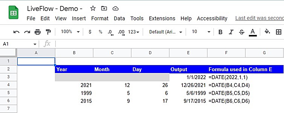
For example, to enter the date January 1, 2022, you would use the following formula:
=DATE(2022, 1, 1)
The function will generate the corresponding date value in the designated cell.
You can also use cell references as parameters in the DATE function for more dynamic date entries. This allows you to input the year, month, and day values from other cells in the spreadsheet. For instance, if the year is stored in cell A1, the month in cell B1, and the day in cell C1, you can use the following formula:
=DATE(A1, B1, C1)
By referencing cells, you can easily update the date by changing the values in those cells without modifying the formula itself.
It’s important to note that the DATE function automatically validates the input and generates a valid date value. Therefore, the function takes care of handling inconsistencies like leap years and varying days in different months.
Using the year, month, and day parameters with the DATE function provides a precise and flexible method for entering dates in Google Spreadsheets. This approach ensures accurate date calculations and simplifies the process of working with date-related data within the spreadsheet.
Using cell references as parameters in the DATE function
One of the powerful features of the DATE function in Google Spreadsheets is the ability to use cell references as parameters. This allows you to dynamically update the date by changing the values in the referenced cells.
When using cell references in the DATE function, you need to substitute the year, month, and day values with references to the respective cells. For example, if the year is stored in cell A1, the month in cell B1, and the day in cell C1, you would use the following formula:
=DATE(A1, B1, C1)
The DATE function will then retrieve the values from the referenced cells and generate the corresponding date value. This approach is particularly useful when you want to link the date calculation to other cells or variables in your spreadsheet.
By using cell references, you can easily update the date by changing the values in the referenced cells. For example, if you decide to change the year from 2022 to 2023, you would only need to update the value in cell A1, and the formula will automatically recalculate the result based on the new input.
This flexibility allows you to build dynamic date calculations that can be easily adjusted without the need to modify the formula itself. It also simplifies working with date-related data that may change over time, such as project timelines or event schedules.
Furthermore, using cell references enhances the efficiency of your spreadsheet. By referencing the same date parameters in multiple formulas, you can ensure consistency across your calculations and avoid the risk of manual errors.
Formatting the date in different styles
Google Spreadsheets provides various options for formatting dates generated using the DATE function. These formatting styles allow you to present the date in a way that is visually appealing and meaningful to you or your audience.
To format a date, you can use the built-in formatting options in Google Spreadsheets. Here are a few common formatting styles:
- Default date format: By default, Google Spreadsheets uses the system settings on your computer to display dates. This format may vary depending on your regional settings, but it commonly uses the day, month, and year order.
- Day, month, and year: This format displays the date as “day/month/year” or “dd/mm/yyyy”. For example, if the date is March 15, 2022, it would be displayed as “15/03/2022”.
- Month, day, and year: This format displays the date as “month/day/year” or “mm/dd/yyyy”. For example, if the date is October 1, 2022, it would be displayed as “10/01/2022”.
- Custom formatting: Google Spreadsheets also allows you to create custom formatting styles for dates. This enables you to define your own format, such as displaying the month as a word instead of a number (e.g., “January 15, 2022”) or including the day of the week (e.g., “Monday, March 15, 2022”).
To apply a formatting style to a date, select the cell containing the date and use the formatting options in the toolbar. You can access these options by clicking on the “Format” menu and choosing “Number” or by using the keyboard shortcut Ctrl+Shift+4.
By formatting the date in different styles, you can make the date information more readable and suitable for your specific needs. Whether you prefer a standard format or a custom format, Google Spreadsheets provides the flexibility to present dates in a way that best represents your data.
Adding or subtracting days, months, or years from a date
The DATE function in Google Spreadsheets not only allows you to generate dates but also enables you to perform calculations by adding or subtracting days, months, or years from a given date. This feature is particularly useful when working with timelines, project schedules, or any analysis involving date-based calculations.
To add or subtract a specific number of days, months, or years from a date, you can use the arithmetic operators (+ or -) combined with the DATE function.
Here’s the general syntax:
=DATE(year, month, day) +/- value
For example, let’s say you have a date in cell A1 and you want to calculate the date that is 7 days later. You can use the following formula:
=A1 + 7
The function will add 7 days to the date in cell A1 and display the new date.
Similarly, you can subtract days by using the subtraction operator. For example, to calculate the date 3 days before the date in cell A1, you can use:
=A1 - 3
In addition to days, you can also add or subtract months or years from a date. For instance, to calculate the date that is 2 months after the date in cell A1, you can use:
=DATE(YEAR(A1), MONTH(A1) + 2, DAY(A1))
This formula extracts the year, month, and day components of the original date using the YEAR, MONTH, and DAY functions, respectively. It then adds 2 to the month and generates the resultant date.
Similarly, you can subtract months or years by subtracting the desired value.
By incorporating addition or subtraction operations with the DATE function, you can perform flexible date calculations and manipulate dates within your Google Spreadsheet to meet your specific requirements.
Calculating the difference between two dates
In Google Spreadsheets, you can easily calculate the difference between two dates using the DATE function. This feature is particularly useful for tracking durations, measuring time intervals, or analyzing the time between two events.
To calculate the difference between two dates, you can subtract the earlier date from the later date. The resulting value will represent the number of days between the two dates.
Here’s the general syntax:
=later_date - earlier_date
For example, let’s say you have the start date in cell A1 and the end date in cell B1. You can calculate the number of days between the two dates using:
=B1 - A1
The function will subtract the value in cell A1 (the earlier date) from the value in cell B1 (the later date) and return the number of days as the result.
If you want to calculate the difference in months or years instead of days, you can use the YEAR and MONTH functions in combination with the DATE function:
=YEAR(later_date) - YEAR(earlier_date) + (MONTH(later_date) - MONTH(earlier_date)) / 12
This formula calculates the difference in years by subtracting the year component of the earlier date from the year component of the later date. It also calculates the difference in months and divides it by 12 to convert it into a fractional year value.
By calculating the difference between two dates, you can gain insights into time intervals, durations, or time-based trends in your spreadsheet. This can be particularly helpful when analyzing project timelines, employee tenure, or any scenario that involves tracking and comparing dates.
Handling errors with the DATE function
While using the DATE function in Google Spreadsheets, there are certain scenarios where you may encounter errors. It’s important to understand these potential pitfalls and how to handle them effectively to ensure accurate and reliable calculations.
Common errors with the DATE function include:
- #VALUE!: This error occurs when one or more of the provided parameters are not valid numbers or cannot be interpreted as numbers. Make sure you input the correct values for the year, month, and day parameters.
- #NUM!: This error occurs when the resulting date is beyond the supported range of dates in Google Spreadsheets. Keep in mind that Google Spreadsheets has a limit on the range of dates it can handle, which typically extends from January 1, 1900, to December 31, 9999.
- #REF!: This error occurs when one or more of the referenced cells used as parameters in the DATE function are deleted or contain invalid data.
To handle these errors, you can take the following steps:
- Verify parameter values: Double-check the input values for the year, month, and day parameters to ensure they are valid numbers or references to cells that contain valid numbers.
- Check for range limits: If you encounter a #NUM! error, verify that the resulting date falls within the supported range of dates. Consider adjusting the input values or using alternative methods for handling dates outside of the supported range.
- Validate referenced cells: If you encounter a #REF! error, ensure that the referenced cells used as parameters in the DATE function exist and contain valid data. If necessary, update the references to valid cells.
If you are unsure about the cause of an error, you can use the error-checking tools in Google Spreadsheets to identify and address any issues. These tools can help you identify formula errors and provide suggestions for resolving them.
By being aware of these potential errors and implementing appropriate error handling techniques, you can ensure the accuracy and reliability of your DATE function calculations in Google Spreadsheets.
Examples of using the DATE function in Google Spreadsheets
The DATE function in Google Spreadsheets is a versatile tool that can be utilized in various scenarios. Let’s explore a few examples to demonstrate how this function can be applied:
- Calculating project due dates: Suppose you have a project with a start date in cell A1 and a duration of 10 days in cell B1. You can use the following formula to calculate the project’s end date:
- Tracking employee tenure: If you have an employee’s hire date in cell A1, you can calculate their length of service in years using:
- Analyzing sales data by month: Suppose you have sales figures for each month in cells A1 to A12, and you want to calculate the average monthly sales. You can use the following formula:
- Generating a dynamic timestamp: If you need to record the current date and time when specific actions occur, you can use the NOW() function combined with the DATE function. For example, the following formula records the current date and time in cell A1:
=A1 + B1
This formula adds the start date with the duration to determine the project’s due date.
=YEAR(TODAY()) - YEAR(A1)
This formula subtracts the hire date’s year from the current year to determine the number of years the employee has been with the company.
=AVERAGE(A1:A12)
This formula calculates the average of the values in cells A1 to A12, representing the monthly sales data.
=NOW()
This formula will update the cell with the current date and time whenever the spreadsheet is recalculated.
These examples demonstrate the versatility and usefulness of the DATE function in Google Spreadsheets. By using this function in combination with other formulas, you can perform calculations, track time-related data, and generate dynamic timestamps to meet your specific needs within the spreadsheet.
Tips and tricks for working with dates in Google Spreadsheets
When working with dates in Google Spreadsheets, there are several tips and tricks you can utilize to maximize efficiency and improve your data management. Here are some valuable tips to consider:
- Use date formatting: Take advantage of Google Spreadsheets’ built-in date formatting options to display dates in a format that is easy to read and understand. You can access formatting options through the “Format” menu or by using keyboard shortcuts.
- Utilize conditional formatting: Apply conditional formatting rules to highlight or format cells based on certain date conditions. For example, you can use conditional formatting to highlight past-due dates or upcoming deadlines.
- Convert text to dates: If you have dates that are stored as text, you can convert them to proper date format using the DATEVALUE function. For example, if the text representation of a date is in cell A1, you can use the formula:
- Extract components of a date: Use the DAY, MONTH, and YEAR functions to extract specific components of a date. For example, if the date is in cell A1, you can use:
- Calculate the number of days between two dates: Subtracting two date values will give you the number of days between them. For instance, if the start date is in cell A1 and the end date is in cell B1, you can use:
- Use the TODAY function: The TODAY function returns the current date. You can utilize this function to incorporate real-time date values in your calculations or conditional formatting. For example, you can compare today’s date with a deadline to determine if it has passed or is upcoming.
- Be mindful of date formats: When working with dates, double-check the formatting to ensure consistency across your spreadsheet. Consider using a consistent date format throughout to avoid confusion and ensure accurate calculations.
=DATEVALUE(A1)
This will convert the text into a valid date format that can be used for calculations or formatting.
=DAY(A1)
=MONTH(A1)
=YEAR(A1)
These functions allow you to extract the day, month, or year value for further calculations or analysis.
=B1 - A1
This calculates the number of days between the start and end dates.
These tips and tricks will help you work with dates more effectively in Google Spreadsheets. They can save you time, improve the accuracy of your calculations, and make your data analysis more efficient and insightful.