
Prerequisites
Before diving into using Google Sheets to reference data from another sheet, there are a few prerequisites to keep in mind. Familiarizing yourself with these key elements will help you make the most of this feature and streamline your data management process.
Firstly, you’ll need a Google account to access Google Sheets. If you don’t already have one, you can easily sign up for a free account on the Google website. Once you have your account, you can access Google Sheets from your web browser or through the Google Sheets mobile app.
Secondly, it’s important to have a basic understanding of how spreadsheets work. If you’re new to spreadsheets, take some time to familiarize yourself with the different components, such as cells, columns, and rows. Understanding how data is organized will make it easier to reference and manipulate data in Google Sheets.
Additionally, a working knowledge of formulas and functions in Google Sheets is essential for referencing data. Formulas allow you to perform calculations and manipulate data within a sheet, while functions are predefined formulas that perform specific tasks. Some commonly used functions for referencing data include VLOOKUP, INDEX, MATCH, and IMPORTRANGE.
Furthermore, it’s helpful to have a clear understanding of the structure and layout of your sheets. Knowing the specific names of the sheets and the range of cells containing the data you want to reference will facilitate the process. Make sure to label your sheets and organize your data in a logical manner to ensure efficient referencing.
Lastly, having a reliable internet connection is crucial, as Google Sheets is a cloud-based platform that requires an internet connection for real-time collaboration and data updates. Without a stable internet connection, it may be difficult to work with and reference data between sheets seamlessly.
By meeting these prerequisites, you’ll be well-prepared to use Google Sheets to reference data from another sheet effectively. Now that you have a solid foundation, we can move on to understanding the various methods and functions for referencing data in Google Sheets.
Understanding Sheets and Spreadsheets
Before we explore how to reference data from another sheet in Google Sheets, it’s important to understand the basic concepts of sheets and spreadsheets. Google Sheets, a web-based spreadsheet program, allows you to create, edit, and store information in a structured manner.
A spreadsheet is a collection of cells organized in rows and columns. Each cell can hold text, numbers, or formulas. Typically, a spreadsheet consists of multiple sheets, which are individual tabs within the spreadsheet. These sheets enable you to organize and categorize your data into separate sections for clarity and ease of access.
When you create a new spreadsheet, Google Sheets automatically provides you with a default sheet named “Sheet1.” However, you can easily add additional sheets by clicking on the “+” icon at the bottom of the spreadsheet. Each sheet can have a unique name that reflects its purpose or the data it contains.
Within a sheet, you can enter data into individual cells. Cells are identified by their column letters and row numbers. For example, the cell in the first column and second row is denoted as A2. You can enter data directly into cells or use formulas and functions to perform calculations and manipulate data automatically.
To navigate between sheets within a spreadsheet, you can either click on the sheet tabs at the bottom of the screen or use the keyboard shortcut Ctrl+PgDn (Windows) or Command+PgDn (Mac). This makes it easy to switch between sheets and reference data from one sheet to another.
Understanding the structure and layout of sheets and spreadsheets is essential for effectively referencing data. By organizing your data into separate sheets and knowing how to access and navigate between them, you can efficiently reference and manipulate data in Google Sheets.
Now that we have a clear understanding of sheets and spreadsheets, let’s dive into creating the source sheet and retrieving data from it in the next sections.
Creating the Source Sheet
To reference data from another sheet in Google Sheets, you first need to create a source sheet that contains the data you want to reference. The source sheet serves as the origin or the “database” of the information you need for calculations, analysis, or other purposes.
To create a new sheet, open your Google Sheets document and click on the “+” icon at the bottom of the screen. Give your sheet a descriptive name that reflects the type of data it will contain. You can also rename the sheet at any time by right-clicking on the sheet tab and selecting “Rename.”
Once you have created your source sheet, you can populate it with the relevant data. Enter the data into the appropriate cells, organizing it in a logical and structured manner. Use headings or labels to clearly identify the different columns and rows and make the data easier to understand.
If you have data in an existing spreadsheet or an external source, you can also import it into your source sheet. To do this, go to the “File” menu and select “Import.” From there, you can choose to import data from other sheets, CSV files, or even tables from websites. Make sure to map the columns correctly to ensure the data is imported accurately.
In addition to basic data entry, Google Sheets provides a range of tools and features to enhance your source sheet. You can apply formatting styles, such as bold or italic, to highlight important information. You can also use data validation to set criteria and restrictions on the data entered into cells.
Remember to save your changes periodically to ensure all the data in your source sheet is up to date. Google Sheets automatically saves your work, but it’s good practice to click on the floppy disk icon in the toolbar to manually save when necessary.
Now that you have created your source sheet and populated it with data, you are ready to reference this data from another sheet. In the following sections, we will explore various methods and functions to retrieve data from the source sheet and use it in different ways.
Retrieving Data from the Source Sheet
Once you have created a source sheet in Google Sheets, the next step is to retrieve the data from this sheet and use it in other sheets or calculations. Retrieving data allows you to access and reference specific information without duplicating it across multiple sheets, saving time and ensuring data consistency.
Google Sheets offers several methods and functions to retrieve data from the source sheet, depending on your specific requirements. Let’s explore some of the common techniques you can use:
One method is to manually copy and paste the data from the source sheet into the destination sheet. This can be done by selecting the desired range of cells in the source sheet, right-clicking, selecting “Copy,” and then navigating to the destination sheet and right-clicking again to select “Paste.” However, this method can be time-consuming, especially if the data in the source sheet frequently changes, as you would need to repeat the copy-paste process each time.
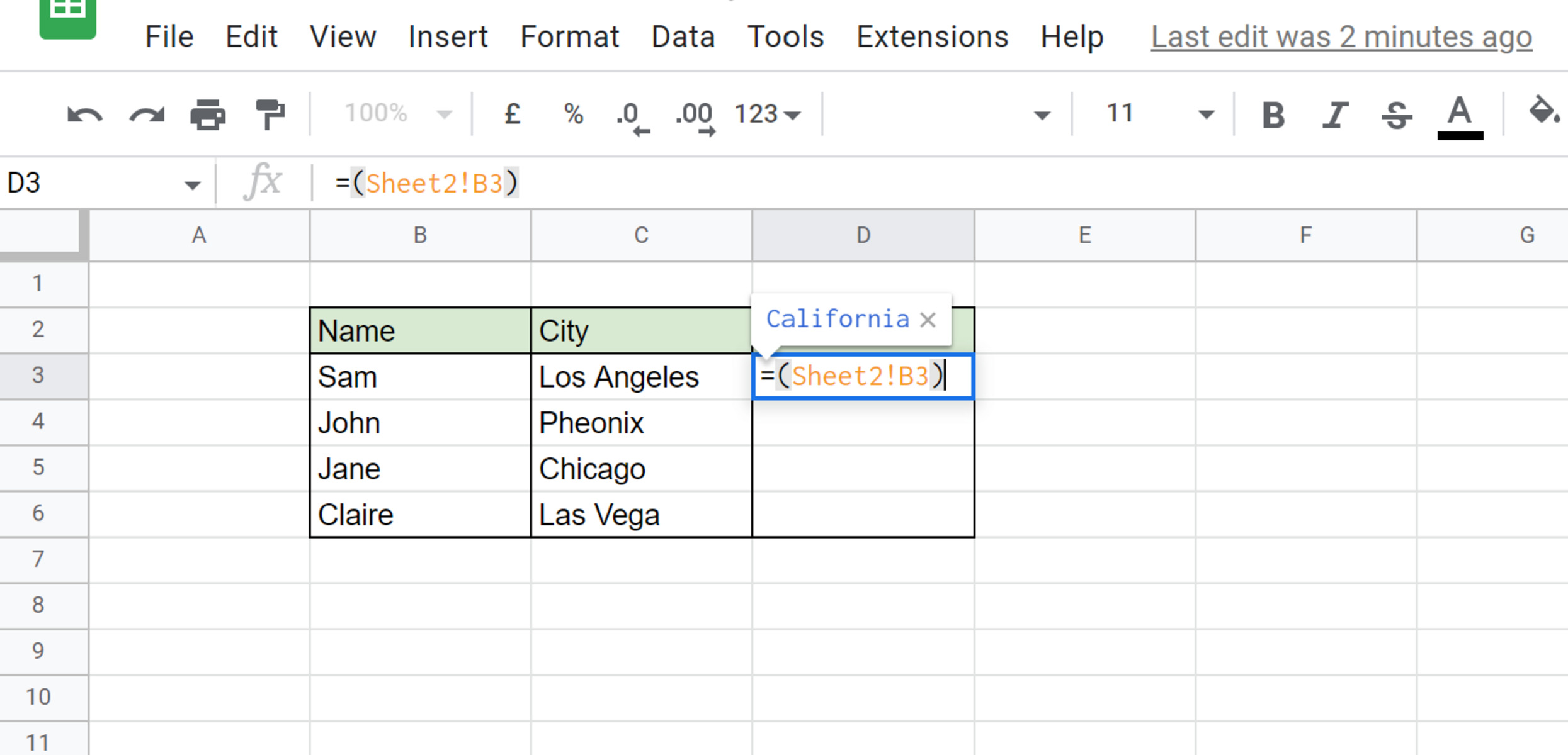
Another method is to use cell references. By referencing the specific cells or ranges in the source sheet, you can automatically retrieve the data in real-time. For example, if you want to reference a cell A1 in the source sheet, you can simply enter “=SheetName!A1” in the destination sheet, replacing “SheetName” with the actual name of the source sheet. This way, any changes made to the value in cell A1 of the source sheet will be automatically reflected in the destination sheet.
In addition to cell references, Google Sheets provides powerful functions such as IMPORTRANGE, QUERY, VLOOKUP, and INDEX-MATCH to retrieve data from the source sheet dynamically. These functions allow you to fetch specific data based on criteria or perform complex calculations using data from multiple sheets. Understanding and utilizing these functions can significantly enhance your data retrieval capabilities in Google Sheets.
Remember to pay attention to the syntax and usage of these functions, as incorrect inputs may result in errors or incorrect data retrieval. The Google Sheets documentation is a valuable resource for learning more about each function and exploring advanced techniques for retrieving data.
By utilizing the various retrieval methods and functions available in Google Sheets, you can efficiently retrieve data from the source sheet and incorporate it into your other sheets or calculations. This allows for better data management, reduces duplication, and ensures the accuracy and consistency of your information across multiple sheets.
Understanding References
In Google Sheets, referencing data from another sheet is a powerful feature that allows you to link and retrieve information from one sheet to another. Understanding how references work is essential for effectively working with multiple sheets and utilizing the data in a seamless manner.
A reference in Google Sheets is a way to identify and connect specific cells, ranges, or even entire sheets within a spreadsheet. By using references, you can dynamically pull data from the source sheet and display it in the destination sheet, ensuring that any changes made to the source data are automatically reflected wherever it is referenced.
There are two main types of references: absolute and relative references. An absolute reference locks the cell or range reference in place, meaning that no matter where it is copied or moved, the reference will always point to the original location. This is denoted by using a “$” symbol before the column letter and row number in the reference. On the other hand, a relative reference adjusts its position when copied or moved. This allows for flexible referencing of nearby cells or ranges.
In addition to cell and range references, Google Sheets also supports sheet references. With sheet references, you can retrieve data from a specific sheet by referencing its name in formulas or functions. This is particularly useful when working with multiple sheets and needing to pull data from a specific sheet without navigating to it manually.
It’s important to note that when referencing data between sheets, the sheet names should be enclosed in single quotation marks (e.g., ‘Sheet1’!A1:B10). This ensures that even if the sheet name contains spaces or special characters, it is correctly recognized by Google Sheets.
Furthermore, references can be combined with various functions to manipulate and analyze the data. Functions like SUM, AVERAGE, COUNT, and more can be used in combination with references to perform calculations on the retrieved data.
By understanding references and utilizing them effectively in your Google Sheets, you can create dynamic connections between different sheets, streamline data management, and ensure the accuracy and consistency of your information across the spreadsheet.
Referencing Data from Another Sheet
Referencing data from another sheet in Google Sheets allows you to access and utilize data from one sheet in a different sheet. This functionality enables you to centralize and organize data in separate sheets while easily referencing and updating it as needed.
To reference data from another sheet, you need to specify the sheet name and the cell or range you want to reference. There are a few ways to accomplish this:
1. Cell Reference: To reference a specific cell from another sheet, use the following syntax: ‘SheetName’!Cell. For example, to reference cell A1 in a sheet named “Data,” you would use the formula ‘=Data!A1’ in the destination sheet. This allows you to pull data from a specific cell into the current sheet.
2. Range Reference: To reference a range of cells from another sheet, use the following syntax: ‘SheetName’!StartCell:EndCell. For example, to reference cells A1 to B5 in the “Data” sheet, you would use the formula ‘=Data!A1:B5’ in the destination sheet. This retrieves all the data within the specified range.
3. Named Range Reference: If you have defined a named range in your source sheet, you can reference it by using the name instead of the cell or range reference. This allows for more flexibility and readability in your formulas. For example, if you have named a range “SalesData” in the “Data” sheet containing cells A1 to B5, you can use ‘=Data!SalesData’ to reference that range.
By leveraging these referencing techniques, you can easily retrieve and use data from another sheet within your Google Sheets. This provides a seamless way to incorporate and analyze data from different sources and maintain data integrity across your spreadsheet.
Furthermore, referencing data is not limited to just one sheet. You can reference data from multiple sheets, allowing you to create complex calculations and analysis using data from different sources. By combining formulas, functions, and referencing techniques, you can perform powerful data manipulations and gain valuable insights.
Remember to update the referenced data whenever changes are made in the source sheet. Google Sheets automatically updates the references in real-time, ensuring that the retrieved data remains accurate and up to date.
Next, we will explore specific functions in Google Sheets that are commonly used to reference data from another sheet, granting you even more control and flexibility in managing and analyzing your data.
Using the IMPORTRANGE Function
The IMPORTRANGE function is a powerful tool in Google Sheets that allows you to import data from one sheet to another. It enables you to establish a dynamic connection between sheets, automatically retrieving and updating data as changes occur in the source sheet. The IMPORTRANGE function is especially useful when referencing data from a different spreadsheet altogether.
To use the IMPORTRANGE function, follow these steps:
1. Identify the source spreadsheet and copy its URL.
2. In the destination sheet, select the cell where you want the imported data to appear.
3. Enter the formula “=IMPORTRANGE(“Source Spreadsheet URL”, “SheetName!Range”)”, replacing “Source Spreadsheet URL” with the copied URL and “SheetName!Range” with the sheet name and range you want to import.
4. Press Enter to import the data.
The IMPORTRANGE function uses a secure connection to access the specified range in the source sheet. However, keep in mind that you must have access to the source spreadsheet in order to import data from it. If the source spreadsheet is not shared with you, you may encounter permission errors.
It’s important to note that the imported data is not linked to the source sheet. Any changes made in the source sheet will not automatically update the imported data in the destination sheet. To update the imported data, you can manually refresh the formula by deleting and re-entering it or using the “Recalculate” option in the “Data” menu.
The IMPORTRANGE function is a versatile tool for referencing data from another sheet, especially when working with data from multiple spreadsheets. It allows you to centralize and integrate data from different sources, streamlining your data analysis and reporting processes.
Additionally, you can combine the IMPORTRANGE function with other formulas and functions to further manipulate and analyze the imported data. By leveraging the power of Google Sheets’ functions, you can perform complex calculations, create dynamic reports, and gain valuable insights from the imported data.
In the next sections, we will explore additional functions in Google Sheets that can be used to reference data from another sheet, expanding your toolkit for data manipulation and analysis.
Importing Data from Another Sheet Using Query
In Google Sheets, the QUERY function is a powerful tool to import data from another sheet and perform advanced data manipulations. It allows you to retrieve specific data based on criteria and conditions, providing more control and flexibility in importing and analyzing data.
To import data from another sheet using the QUERY function, follow these steps:
1. In the destination sheet, select the cell where you want the imported data to appear.
2. Enter the formula “=QUERY(‘Source Sheet Name’!Range, “SELECT * WHERE Condition”)”, replacing ‘Source Sheet Name’ with the name of the sheet you want to import from and ‘Range’ with the range that contains the data you want to import.
3. Within the double quotation marks, define the criteria or conditions for selecting the data using the SQL-like syntax. For example, you can use “SELECT * WHERE A > 100” to import all the rows where the value in column A is greater than 100.
4. Press Enter to import and display the filtered data.
The QUERY function allows you to perform various operations on the imported data, such as sorting, grouping, and aggregating. By including additional clauses in the formula, you can further manipulate and analyze the imported data to suit your needs.
One of the advantages of using the QUERY function is that it provides a dynamic connection to the source sheet. If any changes are made to the data in the source sheet, the imported data in the destination sheet will automatically update to reflect those changes. This ensures that your analysis and reports are always based on the latest data.
It’s worth noting that the QUERY function has a specific syntax, and the criteria or conditions must be constructed correctly to avoid errors. Take some time to familiarize yourself with the syntax of the QUERY function and experiment with different combinations to retrieve the desired data effectively.
By using the QUERY function, you can import data from another sheet and perform complex data manipulations within Google Sheets. This allows for more advanced analysis and reporting capabilities, helping you gain deeper insights from your data.
In the following sections, we will explore additional functions in Google Sheets that can be used to reference data from another sheet, expanding your range of options for data retrieval and analysis.
Using VLOOKUP to Reference Data
VLOOKUP is a commonly used function in Google Sheets for referencing data from another sheet based on a specific criteria or key. It allows you to search for a value in a column and retrieve the corresponding value from a different column within the same row.
To use VLOOKUP to reference data from another sheet, follow these steps:
1. In the destination sheet, select the cell where you want the referenced data to appear.
2. Enter the formula “=VLOOKUP(SearchKey, ‘Source Sheet Name’!Range, ColumnIndex, False)”, replacing ‘SearchKey’ with the value you want to search for, ‘Source Sheet Name’ with the name of the sheet containing the data, ‘Range’ with the range that contains the data, and ‘ColumnIndex’ with the number of the column in the range from which you want to retrieve the data.
3. Press Enter to display the referenced data.
The VLOOKUP function searches for the specified value in the leftmost column of the given range. Once a match is found, it retrieves the corresponding value from the column specified by ‘ColumnIndex’. The ‘False’ argument ensures an exact match, so it’s important to have the values in the leftmost column sorted in ascending order.
VLOOKUP is especially useful when you have a large dataset with a unique identifier (such as an ID or name) that you want to use as a reference to retrieve additional information from another sheet. It simplifies the process of linking related data together without the need for complex formulas or manual copying and pasting.
Keep in mind that if the search key is not found in the leftmost column of the range, VLOOKUP will return an error. To handle this, you can use an IFERROR function to display a specific value or message when an error occurs.
By using VLOOKUP, you can efficiently reference and retrieve data from another sheet in Google Sheets. Whether you’re creating reports, performing data analysis, or managing large datasets, VLOOKUP is a valuable tool for connecting and consolidating data across different sheets.
In the subsequent sections, we will explore additional functions that can be used to reference and cross-reference data in Google Sheets, further expanding your capabilities for data manipulation and analysis.
Using INDEX and MATCH Functions for Cross-Referencing
When it comes to cross-referencing data in Google Sheets, the combination of the INDEX and MATCH functions is a powerful tool. These functions work together to lookup and retrieve data from multiple sheets based on specific criteria, allowing for more flexible and dynamic cross-referencing capabilities.
To use the INDEX and MATCH functions for cross-referencing, follow these steps:
1. In the destination sheet, select the cell where you want the cross-referenced data to appear.
2. Enter the formula “=INDEX(‘Source Sheet Name’!Range, MATCH(SearchKey, ‘Source Sheet Name’!LookupRange, MatchType))”, replacing ‘Source Sheet Name’ with the name of the sheet containing the data, ‘Range’ with the range from which you want to retrieve the data, ‘SearchKey’ with the value you want to match, ‘LookupRange’ with the range in which you want to search for the ‘SearchKey’, and ‘MatchType’ with either 0, 1, or -1, depending on the type of matching you need (exact match, less than or equal to match, or greater than or equal to match).
3. Press Enter to display the cross-referenced data.
The INDEX function retrieves the value from the specified range based on the row and column number. The MATCH function, on the other hand, searches for the specified value in the lookup range and returns the relative position of the value. By combining these two functions, you can locate and retrieve data from another sheet based on specific criteria.
One of the advantages of using INDEX and MATCH for cross-referencing is their flexibility. Unlike VLOOKUP, which only searches for values in the leftmost column, INDEX and MATCH can search and retrieve data from any column within the range. This allows for more complex cross-referencing scenarios and enables you to build dynamic data retrieval systems.
Additionally, INDEX and MATCH are not limited to just one-to-one matches. You can use them to perform one-to-many or many-to-one cross-references by combining them with array formulas or using range intersections.
By leveraging the power of INDEX and MATCH, you can create sophisticated cross-referencing systems in Google Sheets. Whether you need to combine data from multiple sources, perform intricate data lookups, or build dynamic reports, INDEX and MATCH functions provide the flexibility and control you need.
In the following sections, we will explore additional techniques and functions that can aid in referencing and manipulating data in Google Sheets, further expanding your knowledge and capabilities in data analysis and management.
Updating Referenced Data Automatically
One of the key advantages of referencing data in Google Sheets is the ability to update the referenced data automatically. This ensures that any changes made in the source sheet are reflected in the destination sheet without the need for manual intervention. By setting up dynamic references, you can streamline your data management process and maintain data accuracy and consistency.
When you reference data using formulas or functions such as cell references, VLOOKUP, INDEX-MATCH, or QUERY, the referenced data updates in real-time. Any modifications made to the source data, such as adding or deleting rows or changing cell values, are immediately reflected in the destination sheet.
It’s worth noting that while the referenced data updates automatically, the formulas or functions themselves do not. To trigger a recalculation and update of the referenced data, you can force a recalculation by manually editing any cell in the destination sheet that contains the formula or function. Alternatively, you can use the recalculation options available in the “Data” menu to update all formulas in the sheet.
Google Sheets also allows for automatic recalculation based on certain events, such as opening the spreadsheet, making changes to any cell, or modifying specific ranges. You can utilize these recalculation settings to ensure that the referenced data is always up to date without requiring manual intervention.
Another way to automate the updating of referenced data is by using scripts or add-ons. Google Apps Script, a JavaScript-based scripting language, allows you to create custom triggers and functions to automate your workflows. With the help of scripts or add-ons, you can set up timed triggers or event-driven triggers to update the referenced data at specific intervals or when certain conditions are met.
Keeping your referenced data up to date is essential for accurate analysis, reporting, and decision-making. By leveraging the automatic updating capabilities of referenced data in Google Sheets, you can ensure that your information is always current and reliable, saving you time and effort in manual data management.
In the upcoming sections, we will explore troubleshooting tips and best practices for referencing data in Google Sheets, helping you overcome common challenges and optimize your workflow.
Troubleshooting Reference Errors
While referencing data in Google Sheets is a powerful feature, you may encounter errors or issues that prevent the references from working correctly. Troubleshooting reference errors can help you identify and resolve any issues, ensuring the smooth functioning of your data management process. Here are some common reference errors and troubleshooting tips:
1. #REF! Error: This error occurs when a reference is invalid or points to a cell, range, or sheet that no longer exists. To fix this error, check the formula or function that contains the reference and ensure that it is pointing to the correct location.
2. #N/A Error: This error typically occurs when a value being searched for in a lookup function, such as VLOOKUP or INDEX-MATCH, is not found. Double-check the search criteria or key and verify that it exists in the source data.
3. #VALUE! Error: This error indicates that the formula or function cannot perform the desired operation due to invalid data types or incorrect inputs. Verify that the data being used in the reference is in the expected format and meets the requirements of the formula or function.
4. Circular references: Circular references occur when the formula or function refers to the cell that it is located in, creating an infinite loop. To resolve this, review the formulas or functions involved and adjust the references to avoid self-referencing.
5. Permissions issues: If you are referencing data from another sheet or spreadsheet, ensure that you have the necessary permissions to access and view that data. Check the sharing settings of the source sheet or spreadsheet and adjust them if needed.
6. Case sensitivity: Google Sheets distinguishes between uppercase and lowercase letters in sheet names and reference values. Ensure that you are entering references correctly, taking note of any case-sensitive requirements.
7. Invalid range: When using ranges in formulas or functions, ensure that the specified range is valid and does not include blank cells, merged cells, or non-adjacent ranges. These can cause reference errors or unexpected results.
To troubleshoot these reference errors, it can be helpful to review the formulas or functions involved, double-check the data and ranges being referenced, and confirm that all necessary permissions are in place. Additionally, checking the syntax and ensuring data consistency can also help resolve reference errors.
Google Sheets provides error messages and indicators that can assist in identifying and resolving reference errors. Take advantage of these tools to understand the nature of the error and make the necessary adjustments to your references.
By being aware of common reference errors and applying troubleshooting techniques, you can effectively resolve issues and ensure the accuracy and reliability of your referenced data in Google Sheets.
In the next section, we will discuss best practices for referencing data in Google Sheets, helping you optimize your workflow and avoid common pitfalls.
Best Practices for Referencing Data in Google Sheets
To work efficiently and effectively with referenced data in Google Sheets, it’s important to follow some best practices. These practices will not only help you maintain data integrity and accuracy but also optimize your workflow. Here are some key best practices for referencing data in Google Sheets:
1. Use descriptive sheet and range names: Instead of relying solely on cell references, consider giving meaningful names to your sheets and ranges. This makes it easier to understand the purpose and content of the referenced data, especially when working with multiple sheets or complex formulas.
2. Organize your sheets logically: Structure your sheets in a clear and logical manner to facilitate easy referencing. Use sheet tabs to categorize and separate different types of data or sections within your spreadsheet.
3. Use named ranges: Define named ranges for frequently referenced data or specific ranges, such as tables or columns. Named ranges make formulas more readable and allow for easier maintenance when the structure of your sheet changes.
4. Avoid hardcoded values within formulas: Instead of directly entering values within formulas or functions, reference them from a cell or named range. This allows you to update the referenced value from one location, making it easier to maintain and modify formulas in the future.
5. Regularly validate and update references: As your spreadsheet evolves and data changes, regularly review and validate your references to ensure they are still accurate. Update references to reflect any changes in sheets, ranges, or source data.
6. Document your references: When working on complex spreadsheets with multiple references, consider documenting them in a separate sheet or in cell comments. This serves as a reference guide and aids in troubleshooting if any errors occur.
7. Avoid excessive cross-sheet references: While referencing data across sheets is powerful, excessive cross-sheet references can lead to a complicated and error-prone spreadsheet. Whenever possible, consider consolidating data into fewer sheets or using functions like QUERY to retrieve and manipulate data within the sheet itself.
8. Test and verify formulas: Always test your formulas and functions to ensure they provide the expected results. Double-check the accuracy of the referenced data and verify that the formulas are working correctly before relying on them for critical data analysis or reporting.
By following these best practices, you can improve the efficiency and reliability of your referenced data in Google Sheets. Consistent naming conventions, organized sheets, and well-documented references will not only save you time but also make it easier for you and others to understand and work with your spreadsheet.
Incorporating these best practices into your data referencing process will streamline your workflow and minimize errors, allowing you to make the most out of Google Sheets’ capabilities.