Relative, Absolute, and Mixed Cell References in Excel and Sheets

Relative Cell References

When working with spreadsheets, it’s essential to understand the concept of cell references. In Excel and Sheets, cell references allow you to refer to other cells within formulas and functions, making your worksheets dynamic and flexible. One of the types of cell references is known as relative cell references.

Relative cell references are references that change their position relative to the formula when copied to other cells. In simpler terms, they adjust their location based on the position of the formula itself.

For example, let’s say you have a formula in cell B2 that adds the values from cells A1 and A2 together: =A1+A2. If you copy this formula to cell B3, it will automatically adjust to =A2+A3. Here, the cell references A1 and A2 are relative references that change as the formula is copied to different cells.

This ability to adjust relative cell references makes it easier to perform calculations on different sets of data without the need to rewrite the formula for each individual cell. It saves time and makes your worksheets more efficient.

Relative cell references are particularly useful when you have a formula that relies on the values of neighboring cells or when you want to apply the same formula to multiple cells and have it adapt to each specific location.

It’s important to note that relative cell references are denoted by the absence of any special characters before the column and row references. For example, in Excel, A1 is a relative cell reference, while $A$1 is an absolute cell reference where the dollar signs lock the reference to that specific cell.

Understanding how to use relative cell references will greatly enhance your ability to work with formulas and functions in Excel and Sheets. Remember, when you copy a formula with relative cell references to a different cell, the references will adjust their position accordingly. This flexibility makes your worksheets more dynamic and allows you to work with large datasets more efficiently.

Absolute Cell References

In Excel and Sheets, absolute cell references are another type of cell reference that allows you to maintain a fixed reference to a specific cell, regardless of where the formula is copied or moved. This means that when you copy a formula with absolute references, the referenced cell will always remain the same.

To create an absolute cell reference, you need to use the dollar sign ($) before the column and/or row reference. For example, $A$1 is an absolute cell reference, where both the column (A) and the row (1) are fixed.

Let’s say you have a formula in cell B2 that multiplies the value in cell A1 by 10: =A1*10. If you copy this formula to cell B3, the relative reference will adjust to =A2*10. However, if you use an absolute reference $A$1, the formula will always refer to cell A1, regardless of where it’s copied.

Absolute cell references are particularly useful when you want to lock a specific cell or range of cells in a formula. This is commonly used when you have a constant value or a reference to a fixed position that should not change.

Additionally, absolute cell references are handy when you want to apply the same formula to multiple cells but maintain a consistent reference to a specific cell. By using absolute references, you can ensure that the formula always refers to the correct cell, regardless of its relative position.

By mastering the use of absolute cell references, you can have better control over your formulas and ensure the accuracy of your calculations. They allow you to maintain fixed references to specific cells, making your worksheets more reliable and easier to manage.

Mixed Cell References

In addition to relative and absolute cell references, Excel and Sheets also offer the option of using mixed cell references. Mixed cell references allow you to combine both relative and absolute references within a single cell reference.

A mixed cell reference typically has either the row or column fixed, while the other remains relative. To create a mixed cell reference, you use the dollar sign ($) before either the column or the row reference, but not both.

For example, if you have a formula in cell B2 that subtracts the value in cell A$1 from the value in cell $A2, the mixed cell reference would be $A2-A$1. Here, the column reference before the dollar sign remains relative (A), while the row reference after the dollar sign remains fixed ($1).

By utilizing mixed cell references, you can have greater control over which parts of the cell reference should stay fixed and which should adjust when the formula is copied or moved. This flexibility enhances your ability to work with complex formulas and calculations.

Mixed cell references are particularly useful when you have a scenario where you want to maintain the fixed reference in one direction, such as across rows or down columns, while allowing the other direction to adjust dynamically. This allows you to apply a consistent formula to multiple rows or columns while taking into account the relative positions of the cells.

Using mixed cell references can greatly simplify your formulas and make them more efficient. They allow you to strike a balance between the flexibility of relative references and the stability of absolute references, giving you the best of both worlds.

By mastering the use of mixed cell references, you can create dynamic and robust formulas in Excel and Sheets. They provide a powerful tool to handle complex calculations and make your worksheets more adaptable to changes.

What are Cell References in Excel?

In Excel, cell references are used to refer to specific cells or ranges of cells within a worksheet. They play a crucial role in creating formulas, functions, and calculations. A cell reference can be thought of as a placeholder that represents the value or data contained in a particular cell.

In Excel, each cell is identified by a combination of a column letter and a row number. For example, cell A1 refers to the first cell in the first column of the worksheet.

Cell references can be categorized into three main types: relative, absolute, and mixed.

Relative Cell References: Relative cell references are references that change their position relative to the formula when copied or moved. They adjust their location based on the position of the formula itself. For example, if you copy a formula with relative references one cell down, the references will adjust accordingly.

Absolute Cell References: Absolute cell references, on the other hand, are references that remain fixed regardless of where the formula is copied or moved. They are denoted by dollar signs ($) before the column and/or row reference. Absolute references are useful when you want a specific cell to always be referred to, no matter the formula’s location.

Mixed Cell References: Mixed cell references combine both relative and absolute references within a single cell reference. You can fix either the row or column while allowing the other to adjust. This allows for greater flexibility and control over the formula’s behavior.

Cell references are the building blocks of Excel formulas and functions. They allow you to perform calculations, manipulate data, and automate tasks within your worksheet. By understanding the different types of cell references and how they behave, you can effectively create powerful and dynamic worksheets.

Whether you’re performing complex calculations or simply organizing data, cell references are an essential concept that underlies the functionality of Excel. They enable you to work with data in a structured and logical manner, allowing for efficient data analysis and decision-making.

What are Cell References in Sheets?

In Google Sheets, cell references work similarly to Excel and are used to refer to specific cells or ranges of cells within a worksheet. These references are essential for creating formulas, performing calculations, and analyzing data. Understanding how cell references function in Sheets is crucial for effectively working with data.

Just like in Excel, each cell in Google Sheets is identified by a combination of a column letter and a row number. For instance, cell A1 refers to the first cell in the first column of the worksheet.

In Sheets, there are three main types of cell references: relative, absolute, and mixed.

Relative Cell References: Relative cell references adjust their position based on the formula’s location when copied or moved to other cells. For example, if you have a formula in cell B2 that references cell A1, when copied to cell B3, the reference will automatically adjust to A2.

Absolute Cell References: Absolute cell references remain fixed regardless of where the formula is copied or moved within the sheet. They are denoted with a dollar sign ($) before the column and/or row reference. Absolute references are useful when you need to refer to a specific cell consistently.

Mixed Cell References: Mixed cell references combine both relative and absolute references within a single cell reference. You can fix either the row or column while allowing the other to adjust. This provides flexibility when applying formulas to different cells.

Cell references in Sheets allow you to perform various calculations, manipulate data, and create dynamic worksheets. By understanding the different types of cell references and their behavior, you can efficiently analyze data and make informed decisions.

Google Sheets provides a user-friendly interface for working with cell references. Whether you are creating formulas, analyzing data, or collaborating with others, understanding how to use cell references will greatly enhance your skills in Sheets.

By utilizing cell references effectively, Sheets offers powerful data analysis capabilities, allowing you to automate calculations, create reports, and explore data trends. With the ability to reference and manipulate data across cells, Sheets becomes a valuable tool for organizing and analyzing information.

How to use Relative Cell References in Excel

Relative cell references in Excel allow you to create formulas that adapt and adjust based on their location when copied or moved. This flexibility is incredibly useful when working with large datasets or when you want to apply the same formula to multiple cells.

To use relative cell references in Excel, follow these steps:

Select the cell where you want to enter the formula.
Type an equal sign (=) to indicate that you are entering a formula.
Refer to the cells you want to include in your formula by simply typing their cell references. For example, to add the values in cells A1 and A2, you would enter =A1+A2 into the formula cell.
Press Enter to calculate the formula and display the result.

Once you have entered the formula using relative cell references, you can easily copy or drag the formula to other cells. The references in the formula will adjust automatically based on their relative positions.

For example, if you copy the formula =A1+A2 from cell B1 to cell B2, it will automatically adjust to =A2+A3, and so on.

Relative cell references are particularly useful when you have formulas that rely on the values of neighboring cells or when you need to perform calculations on different sets of data. Instead of rewriting the formula for each individual cell, you can simply copy it and let the references adjust automatically.

By mastering the use of relative cell references, you can expedite your data analysis and make your worksheets more efficient. They provide a dynamic way to work with formulas in Excel, allowing you to automate calculations and handle large datasets with ease.

How to use Relative Cell References in Sheets

Relative cell references in Google Sheets allow you to create formulas that dynamically adjust their references based on their location when copied or moved. This flexibility is invaluable when working with data and performing calculations across multiple cells.

To use relative cell references in Sheets, follow these steps:

Select the cell where you want to enter the formula.
Begin the formula by typing an equal sign (=).
Refer to the cells you want to include in your formula by typing their cell references. For example, to add the values in cells A1 and A2, you would enter =A1+A2 into the formula cell.
Press Enter to calculate the formula and display the result.

Once you have entered the formula using relative cell references, you can easily copy or drag the formula to other cells. The references in the formula will automatically adjust based on their relative positions.

For example, if you copy the formula =A1+A2 from cell B1 to cell B2, it will automatically adjust to =A2+A3, and so on.

Relative cell references are particularly useful when you have formulas that depend on the values of neighboring cells or when you want to apply the same formula to multiple cells. Instead of rewriting the formula for each cell, you can copy it and let the references adapt automatically.

By mastering the use of relative cell references in Sheets, you can streamline your workflow and make your data analysis more efficient. They provide a dynamic approach to working with formulas, enabling you to automate calculations and handle large datasets with ease.

How to use Absolute Cell References in Excel

Absolute cell references in Excel allow you to create formulas that always refer to a specific cell, regardless of where they are copied or moved. This is particularly useful when you need to maintain a fixed reference in your formulas, such as when working with constants or using a reference cell as a point of comparison.

To use absolute cell references in Excel, follow these steps:

Select the cell where you want to enter the formula.
Begin the formula by typing an equal sign (=).
Fix the row and/or column reference of the cell you want to refer to by adding dollar signs ($) before the column letter and/or row number. For example, if you want to refer to cell A1 as an absolute reference, you would enter $A$1 into the formula.
Press Enter to calculate the formula and display the result.

Once you have entered the formula using absolute cell references, you can copy or move the formula to other cells, and the referenced cell will always remain the same. The dollar sign locks the reference to its specific cell.

For example, if you copy a formula with an absolute reference from cell B1 to cell B2, it will still refer to cell A1, as indicated by the absolute reference $A$1.

Absolute cell references are particularly useful when you want to refer to a constant value that should not change, or when you want to keep the reference cell fixed as a point of comparison in your formulas. They ensure the accuracy and consistency of your calculations, regardless of the formula’s location.

By utilizing absolute cell references effectively, you can have better control over your formulas and make your worksheets more reliable. They allow you to fix specific cell references, making your calculations more robust and reducing the chances of errors.

How to use Absolute Cell References in Sheets

Absolute cell references in Google Sheets allow you to create formulas that always reference a specific cell, regardless of where they are copied or moved. By using dollar signs ($) before the column letter and/or row number, you can fix a cell reference and ensure its value remains constant.

To use absolute cell references in Sheets, follow these steps:

Select the cell where you want to enter the formula.
Begin the formula by typing an equal sign (=).
Fix the row and/or column reference of the cell you want to refer to by adding dollar signs ($) before the column letter and/or row number. For example, if you want to refer to cell A1 as an absolute reference, you would enter $A$1 into the formula.
Press Enter to calculate the formula and display the result.

For example, if you copy a formula with an absolute reference from cell B1 to cell B2, it will still refer to cell A1, as indicated by the absolute reference $A$1.

Absolute cell references are particularly useful when you want to maintain a fixed reference to a specific cell in your formulas. They ensure consistency and accuracy, especially if you have constants or reference cells that should not change with the formula’s location.

How to use Mixed Cell References in Excel

Mixed cell references in Excel allow you to combine both relative and absolute references within a single cell reference. This provides you with the flexibility to fix either the row or column while allowing the other to adjust when the formula is copied or moved. Mixed cell references are particularly useful when you want to maintain a fixed reference in one direction while allowing flexibility in the other.

To use mixed cell references in Excel, follow these steps:

Select the cell where you want to enter the formula.
Begin the formula by typing an equal sign (=).
Fix either the row or column reference by adding a dollar sign ($) before it, while leaving the other part of the reference without a dollar sign. For example, if you want to fix the column reference to A but allow the row reference to adjust, you would enter $A1 into the formula.
Press Enter to calculate the formula and display the result.

Once you have entered the formula using mixed cell references, you can copy or move it to other cells. The referenced cell will adjust in the flexible direction while remaining fixed in the other direction.

For example, if you copy a formula with a mixed reference from cell B1 to cell B2, the column reference will remain locked as A ($A1), but the row reference will adjust as B ($A2).

Mixed cell references are particularly useful when you want to maintain a consistent reference to a specific cell in one direction, while allowing flexibility in the other direction. This enables you to apply the same formula to multiple rows or columns, taking into account the relative positions of the cells.

By mastering the use of mixed cell references, you can create powerful and flexible formulas in Excel. They give you the ability to control how your formulas adapt when copied or moved, allowing for efficient data analysis and calculations within your worksheets.

How to use Mixed Cell References in Sheets

Mixed cell references in Google Sheets allow you to combine both relative and absolute references within a single cell reference. By fixing either the row or column reference while allowing the other to adjust, you can create formulas that adapt dynamically while maintaining a fixed reference in a specific direction.

To use mixed cell references in Sheets, follow these steps:

Select the cell where you want to enter the formula.
Begin the formula by typing an equal sign (=).
Fix either the row or column reference by adding a dollar sign ($) before it, while leaving the other part of the reference without a dollar sign. For example, if you want to fix the column reference to A but allow the row reference to adjust, you would enter $A1 into the formula.
Press Enter to calculate the formula and display the result.

For example, if you copy a formula with a mixed reference from cell B1 to cell B2, the column reference will remain locked as A ($A1), but the row reference will adjust as B ($A2).

Mixed cell references are particularly useful in scenarios where you want to maintain a consistent reference in one direction while allowing flexibility in the other direction. This allows you to apply a formula consistently to multiple rows or columns, taking into account the relative positions of the cells.

By mastering the use of mixed cell references in Sheets, you can create dynamic and flexible formulas. They give you the ability to control your formulas’ behavior when copied or moved, allowing for efficient data analysis and calculations within your worksheets.

Tips and Tricks for using Cell References in Excel

Working with cell references in Excel can greatly enhance your ability to create powerful formulas and perform complex calculations. To make the most out of cell references, consider the following tips and tricks:

Use named ranges: Instead of using cell references directly in your formulas, assign a name to a range of cells. This will make your formulas more readable and easier to understand, especially for complex worksheets.
Use absolute references in locked cells: If you want to lock specific cells from being edited, use absolute cell references to refer to those cells in formulas. This ensures that the formulas keep referring to the locked cells even if other parts of the worksheet are modified.
Use relative references for dynamic calculations: When creating formulas that need to adjust cell references based on relative positions, utilize relative cell references. This allows formulas to be copied or moved around the worksheet without the need to manually adjust the references.
Be mindful of row and column references: Ensure that you choose the correct row and column references in your formulas. Mistakenly using the wrong reference can lead to incorrect calculations and errors in your data analysis.
Document your formulas: As your worksheets become more complex, document your formulas with comments. This helps you and others understand the purpose and logic behind the formulas used.
Validate your formulas: Regularly check the results of your formulas to ensure they are accurate and producing the expected output. This is especially important when working with large datasets or complex calculations.
Utilize the Evaluate Formula feature: If you encounter errors or need to troubleshoot your formulas, utilize the “Evaluate Formula” feature in Excel. This helps you step through the formula and see how Excel is evaluating each part.
Take advantage of autofill and shortcuts: Excel offers powerful autofill features that allow you to quickly populate formulas across a range of cells. Use keyboard shortcuts like Ctrl + D to fill down or Ctrl + R to fill right, saving you time and effort when working with repetitive formulas.

By applying these tips and tricks, you can maximize the efficiency and accuracy of your formulas and make the most out of cell references in Excel. These methods will help you streamline your workflow, simplify complex calculations, and improve the overall functionality of your worksheets.

Tips and Tricks for using Cell References in Sheets

Utilizing cell references effectively in Google Sheets can greatly enhance your ability to perform calculations, analyze data, and organize information. To optimize your use of cell references, consider the following tips and tricks:

Use named ranges: Assigning names to specific ranges of cells can make your formulas more readable and easier to understand. It also allows for easier navigation within your spreadsheet.
Combine relative and absolute references: Use mixed cell references to fix either the row or column while allowing the other to adjust. This provides flexibility in formulas and allows for dynamic calculations when copying or moving them.
Choose descriptive cell references: When creating formulas, choose cell references that are clear and descriptive. This makes it easier for you and others to understand the logic and purpose of the formula.
Document your formulas: Add comments to your formulas to explain their purpose and any specific information relevant to them. This helps you and others understand and troubleshoot formulas in the future.
Use the Explore feature: Google Sheets offers the Explore feature, which utilizes artificial intelligence to suggest data analysis options and formulate formulas based on your data. Take advantage of this feature to simplify your data analysis process.
Learn keyboard shortcuts: Using keyboard shortcuts in Sheets can greatly improve your efficiency and speed. Familiarize yourself with shortcuts like Ctrl + D to fill down or Ctrl + R to fill right, saving you time when working with formulas.
Utilize the ARRAYFORMULA function: The ARRAYFORMULA function allows you to apply a formula to an entire range of cells, eliminating the need to manually enter the formula in each cell. This can be especially useful when working with large datasets.
Test and validate your formulas: Regularly test your formulas to ensure they produce accurate results. Double-check the output against expected values and adjust the formulas as needed.

By implementing these tips and tricks, you can streamline your workflow, improve the accuracy of your calculations, and make the most of cell references in Google Sheets. These techniques will help you analyze data efficiently, create dynamic formulas, and optimize your productivity when working with spreadsheets.

Examples of using Cell References in Excel

Cell references in Excel are fundamental to creating formulas and performing calculations. They allow you to refer to specific cells or ranges of cells, enabling dynamic and flexible data analysis. Here are a few examples of how to use cell references in Excel:

Summing a range of values: To calculate the sum of values in a range, use the SUM function along with a cell reference that specifies the range. For example, =SUM(A1:A5) will sum the values in cells A1 to A5.
Referencing cells in another sheet: When referencing cells in a different sheet, use the sheet name followed by an exclamation mark (!), then the cell reference. For instance, =Sheet2!A1 refers to cell A1 in Sheet2.
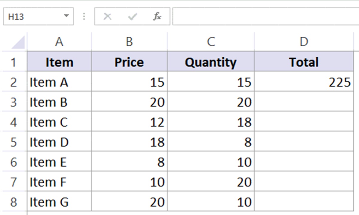
Performing calculations based on relative positions: If you have a series of values in column A and want to calculate a percentage based on each value, use a relative cell reference. For example, =A1/A$1 will divide the value in each cell by the value in cell A1.
Using calculations with mixed cell references: Suppose you have a table with prices in column A and quantities in column B, and you want to calculate the total cost in column C. To multiply the price by the quantity, use the mixed cell reference =A2*$B$2 and copy the formula down to calculate the total cost for each row.
Using absolute cell references in formulas: If you have a fixed tax rate stored in cell B1 and want to calculate the total cost including tax, use an absolute cell reference. For example, =A1+($A1*$B$1) will add the value in cell A1 to the product of cell A1 and the tax rate in cell B1.

These examples illustrate how cell references can be used in various scenarios in Excel. Whether you are performing simple calculations or analyzing complex datasets, understanding how to use cell references effectively is crucial for accurate and efficient data analysis in Excel.

Examples of using Cell References in Sheets

Using cell references in Google Sheets allows you to perform calculations, analyze data, and create dynamic worksheets. Here are a few examples of how to use cell references in Sheets:

Calculating the average: To calculate the average of a range of values, use the AVERAGE function along with a cell reference that specifies the range. For example, =AVERAGE(A1:A5) will give you the average of the values in cells A1 to A5.
Referring to cells in other sheets: When referencing cells in a different sheet, use the sheet name followed by an exclamation mark (!), then the cell reference. For instance, =Sheet2!A1 refers to cell A1 in Sheet2.
Performing calculations based on relative positions: If you have a series of values in column A and want to calculate a percentage change based on each value, use a relative cell reference. For example, =(A2-A1)/A1 will calculate the percentage change from the previous cell in column A.
Using calculations with mixed cell references: Suppose you have a table with prices in column A and quantities in column B, and you want to calculate the total cost in column C. To multiply the price by the quantity, use the mixed cell reference =A2*B$2 and copy the formula down to calculate the total cost for each row.
Using absolute cell references in formulas: If you have a constant value or a reference cell that you want to keep fixed, use an absolute cell reference. For example, =A1*$B$1 will multiply the value in cell A1 by the fixed value in cell B1.

These examples demonstrate how cell references can be used in Google Sheets to perform calculations and analyze data. By leveraging cell references, you can easily apply formulas to multiple cells, create dynamic calculations, and make your worksheets more efficient and adaptable to changes.

Common Mistakes to Avoid when using Cell References in Excel

Working with cell references in Excel can sometimes lead to errors if not utilized correctly. Here are some common mistakes to avoid when using cell references:

Using incorrect cell references: Double-check that you are referencing the correct cells in your formulas. Typos or selecting the wrong range can result in inaccurate calculations.
Forgetting to lock cell references: If you need to fix a specific cell reference in a formula, make sure to use absolute references by adding dollar signs ($) before the column and/or row references. Neglecting to do so can lead to unintended changes when the formula is copied or moved.
Mixing up relative and absolute references: In complex formulas or ranges, ensure that you are using the appropriate type of cell references. Mixing up relative and absolute references can produce incorrect results.
Not adjusting references when inserting/deleting rows or columns: When inserting or deleting rows or columns within a range referenced by a formula, ensure that you update the formula and adjust the references accordingly.
Referencing cells on different sheets without specifying the sheet name: When referencing cells on different sheets, always include the sheet name followed by an exclamation mark (!) to avoid referencing the wrong cells.
Not using parentheses for complex calculations: When performing complex calculations with multiple operations, use parentheses to ensure the desired order of calculations. Failing to do so may cause incorrect results.
Copying/pasting formulas without reviewing the references: Before copying or pasting formulas across cells or worksheets, review the references to ensure they adjust or stay fixed correctly depending on your intention.

By being mindful of these common mistakes, you can avoid errors and ensure the accuracy and reliability of your formulas. Regularly double-checking your formulas and understanding how cell references work will greatly enhance the quality of your analyses and calculations in Excel.

Common Mistakes to Avoid when using Cell References in Sheets

Working with cell references in Google Sheets can lead to errors if not used correctly. Here are some common mistakes to avoid when using cell references:

Using incorrect cell references: Double-check that you are referencing the correct cells in your formulas. Accidentally selecting the wrong range or mistyping the cell references can result in inaccurate calculations.
Forgetting to lock cell references: If you need to fix a specific cell reference in a formula, make sure to use absolute references by adding dollar signs ($) before the column and/or row references. Neglecting to do so can lead to unintended changes when the formula is copied or moved.
Mixing up relative and absolute references: Ensure that you are using the appropriate type of cell references in your formulas. Mixing up relative and absolute references can produce incorrect results.
Not adjusting references when inserting/deleting rows or columns: When you insert or delete rows or columns within a range referenced by a formula, ensure that you update the formula and adjust the references accordingly.
Referencing cells on different sheets without specifying the sheet name: When referencing cells on different sheets, always include the sheet name followed by an exclamation mark (!) to avoid referencing the wrong cells.
Not using parentheses for complex calculations: When performing complex calculations with multiple operations, use parentheses to ensure the desired order of calculations. Failing to do so may cause incorrect results.
Copying/pasting formulas without reviewing the references: Before copying or pasting formulas across cells or sheets, review the references to ensure they adjust or remain fixed correctly based on your intended logic.

By being cautious of these common mistakes, you can avoid errors and ensure the accuracy and reliability of your formulas in Google Sheets. Regularly reviewing and verifying your formulas, along with understanding how cell references work, will significantly enhance the quality of your data analysis and calculations.