
What is the MONTH Formula?
The MONTH formula is a powerful function in Microsoft Excel that allows you to extract the month component from a given date. It is particularly useful when you want to perform calculations or analysis based on the month alone, without considering the day or year.
The MONTH formula belongs to the category of Date & Time functions in Excel. It takes a date as input and returns the corresponding month as a number between 1 and 12. This numeric representation makes it easier for you to work with dates and perform various operations.
Using the MONTH formula, you can extract the month from a date and use it for a variety of purposes. For example, you can analyze sales data based on monthly performance, calculate the average monthly expenses, or filter data based on a specific month.
By understanding and utilizing the MONTH formula, you can enhance your data analysis skills in Excel and streamline your workflow. Whether you are a business professional, a student, or an avid Excel user, this formula can greatly simplify your tasks and improve your efficiency.
Next, let’s explore the syntax of the MONTH formula and learn how to use it effectively in Excel.
Syntax of the MONTH Formula
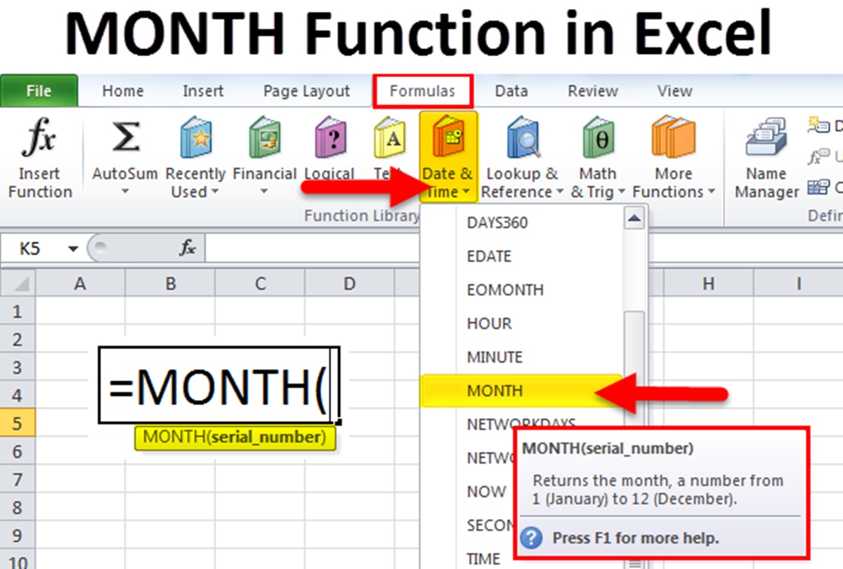
The syntax of the MONTH formula is quite simple and straightforward. It follows the standard structure of Excel formulas:
=MONTH(serial_number)
The serial_number is the date from which you want to extract the month. It can be entered directly as a date in quotation marks, or it can be a reference to a cell containing a date.
For example, if you want to extract the month from the date stored in cell A1, you would use the formula:
=MONTH(A1)
The formula will return the month as a number between 1 and 12, corresponding to January to December.
It is important to note that the MONTH formula only works with valid dates recognized by Excel. If the input date is not recognized as a valid date, the formula will return an error.
Now that you understand the syntax of the MONTH formula, let’s move on to some practical examples to illustrate how it can be used in different scenarios.
Examples of Using the MONTH Formula
The MONTH formula can be used in various scenarios to extract and manipulate the month component of a date. Let’s explore some practical examples:
Example 1: Extracting the Month from a Date
Suppose you have a sales dataset with a column containing the dates of each sale. You want to extract the month from each date to analyze the monthly sales performance. You can use the MONTH formula as follows:
=MONTH(A2)
This formula assumes that the date is stored in cell A2. Copy the formula down the column to extract the month for each sale date. Now you have a separate column with the month component, which can be used for further analysis.
Example 2: Extracting the Month as a Number
In some cases, you may need the month component as a number rather than as the name of the month. For example, you want to identify the months with the highest and lowest sales. You can use the MONTH formula within other functions, such as MAX or MIN, to achieve this:
=MAX(MONTH(A2:A100))
This formula will return the highest month number from the range A2:A100, allowing you to determine the month with the maximum sales. Similarly, you can use the MIN function to find the month with the lowest sales.
Example 3: Working with Dates in Different Formats
Excel recognizes dates in various formats, such as “dd/mm/yyyy” or “mm/dd/yyyy”, based on the regional settings of your computer. If you are working with dates in a different format, you can use the DATE function to convert them to a recognizable format before applying the MONTH formula.
Example 4: Calculating the Month Difference between Two Dates
The MONTH formula can also be used to calculate the difference in months between two dates. For example, you want to determine the number of months it took to complete a project by subtracting the start date from the end date. You can use the DATEDIF function in combination with the MONTH formula:
=DATEDIF(A2, B2, “m”)
This formula calculates the difference in months between the dates in cells A2 and B2. The “m” argument specifies that the result should be in months.
These examples demonstrate the versatility and usefulness of the MONTH formula in Excel. By understanding its application in different scenarios, you can harness the power of this formula to analyze and manipulate date data effectively.
Extracting the Month from a Date
One of the most common and straightforward uses of the MONTH formula is to extract the month from a given date. This can be useful when you want to analyze or categorize data based on monthly values. Here’s how you can extract the month from a date using the MONTH formula:
Let’s say you have a dataset with a column containing various dates. To extract the month for each date, you can use the MONTH formula as follows:
=MONTH(A2)
In this formula, A2 represents the cell containing the date that you want to extract the month from. It will return the month as a number between 1 and 12, representing January to December, respectively.
Copy the formula down the column, and you will have the month component extracted for each date in the dataset. This makes it easier for you to analyze and compare data based on monthly values.
For example, you can use the extracted month to calculate the total sales for each month, identify the months with the highest or lowest sales, or create a pivot table to summarize data by month.
It’s worth noting that when you extract the month component using the MONTH formula, it only takes into account the month and not the day or year. This can be particularly helpful when you want to focus on analyzing trends or patterns based on the month alone.
By utilizing the MONTH formula to extract the month from a date, you can streamline your data analysis process and gain valuable insights into the behavior and performance of your data on a monthly basis.
Extracting the Month as a Number
While the MONTH formula extracts the month component from a date, it returns the month as a number between 1 and 12. This numeric representation can be useful in various situations where you need to work with the month as a numerical value rather than the name of the month. Here’s how you can extract the month as a number using the MONTH formula:
Suppose you have a dataset with dates, and you want to identify the months with the highest and lowest sales. You can use the MONTH formula in combination with other functions, such as MAX or MIN, to achieve this:
=MAX(MONTH(A2:A100))
In this example, A2:A100 represents the range of cells containing the dates. By applying the MONTH formula within the MAX function, you can determine the highest month number within the given range. This provides you with the month with the maximum sales.
Similarly, you can use the MIN function to find the month with the lowest sales:
=MIN(MONTH(A2:A100))
This formula will return the month number with the minimum sales. By identifying the highest and lowest months as numbers, you can easily compare and analyze the performance of different months in your dataset.
Working with the month as a number brings flexibility in performing calculations and comparisons based on the numeric value. It enables you to take advantage of mathematical operations and logical functions like IF, SUMIF, and COUNTIF to further analyze and manipulate your data.
By extracting the month as a number using the MONTH formula, you can gain insights into monthly patterns, trends, and variations in your data, allowing you to make informed decisions and take appropriate actions.
Working with Dates in Different Formats
Excel recognizes dates in various formats, depending on the regional settings of your computer. However, working with dates in different formats can sometimes pose challenges when using functions like the MONTH formula. Fortunately, Excel provides the flexibility to handle dates in different formats and convert them to a recognizable format. Here’s how you can work with dates in different formats:
Converting Text to Date Format:
If your dates are formatted as text, you will need to convert them to a recognizable date format before applying the MONTH formula. To do this, you can use the DATEVALUE function.
For example, if your dates are in the format “dd/mm/yyyy”, and Excel recognizes them as text, use the following formula:
=DATEVALUE(A2)
In this formula, A2 represents the cell containing the date in text format. Excel will convert the text into a recognizable date format that can be used with the MONTH formula.
Changing Date Format:
If Excel is not recognizing your dates in the desired format, you can change the date format using the cell formatting options. Select the range containing the dates, right-click, and choose “Format Cells.” From there, you can select the desired date format, such as “dd/mm/yyyy” or “mm/dd/yyyy”. Excel will then recognize and interpret the dates accordingly.
Using the DATE Function:
If you have dates represented by separate day, month, and year values, you can use the DATE function to combine them into a valid date format. For example, if the day is in cell A1, the month is in cell B1, and the year is in cell C1, you can use the following formula:
=DATE(C1, B1, A1)
This formula will create a valid date based on the day, month, and year values provided. You can then use this date with the MONTH formula to extract the month component.
By effectively handling dates in different formats, you can ensure that the MONTH formula accurately extracts the month component and allows you to work with dates in your preferred format.
Calculating the Month Difference between Two Dates
The MONTH formula can also be used to calculate the difference in months between two dates. This can be handy when you need to determine the duration or interval between two specific points in time. Here’s how you can calculate the month difference between two dates using the MONTH formula:
Suppose you have a project management dataset, and you want to determine the number of months it took to complete a project. You have the start date in cell A2 and the end date in cell B2. To calculate the month difference, you can use the DATEDIF function in combination with the MONTH formula:
=DATEDIF(A2, B2, “m”)
In this formula, A2 represents the start date, and B2 represents the end date. The “m” argument specifies that the result should be in months.
The DATEDIF function calculates the difference in months between the two dates and returns the result as a numeric value. This allows you to determine the number of months it took to complete the project.
It’s important to note that the DATEDIF function is a hidden function in Excel, which means it won’t appear in the function list. However, you can still use it by typing the function directly into the formula bar.
In addition, when using the DATEDIF function, it’s crucial to ensure that the start date is earlier than the end date. Otherwise, the formula might return unexpected results.
By calculating the month difference between two dates, you can accurately measure the duration of a project, track the time elapsed between two milestones, or determine the period between any other significant events.
Utilizing the MONTH formula in conjunction with the DATEDIF function facilitates effective time analysis and enables you to make data-driven decisions based on the duration between specific dates.
Handling Errors with the MONTH Formula
When working with the MONTH formula in Microsoft Excel, it is important to be aware of potential errors that may occur. Understanding how to handle these errors can help ensure the accuracy and reliability of your calculations. Here are some common error scenarios and ways to handle them:
Error Handling for Invalid Dates:
If the input date provided to the MONTH formula is not recognized as a valid date, Excel will return an error. This can happen if the date is typed incorrectly or if the cell contains text instead of a date value.
To handle this error, you can use the IFERROR function to display a custom message or value instead of the error. For example:
=IFERROR(MONTH(A2), “Invalid Date”)
In this formula, A2 represents the cell containing the date. If the date is invalid, the formula will display the message “Invalid Date” instead of the error. You can tailor the custom message to suit your specific needs.
Error Handling for Empty Cells:
If the cell reference in the MONTH formula is empty, Excel will return a #VALUE! error. This can occur if the cell intended to contain a date is left blank.
To handle this error, you can use the IF function to check if the cell is empty before applying the MONTH formula. For example:
=IF(A2=””, “”, MONTH(A2))
In this formula, A2 represents the cell containing the date. If the cell is empty, the formula will display an empty value (“”) instead of the error.
By handling errors with the MONTH formula, you can prevent unexpected results, improve the accuracy of your calculations, and enhance the user experience of your spreadsheets.
Remember to always validate and verify inputs to ensure that they are in the correct format and suitable for use with the MONTH formula. Additionally, employing error handling techniques can lead to smoother data analysis and more reliable results in Excel.