Serial Number and Serial Date in Excel

What is a Serial Number in Excel?

A serial number in Excel is a consecutive number or identifier assigned to a set of data or entries in a column. It is commonly used to establish a unique identity for each record or item in a list or database. Serial numbers play a critical role in organizing, sorting, and manipulating data in Excel spreadsheets.

Excel assigns a serial number to each cell based on the position of the cell within a column or row. The serial number follows a sequential pattern, starting from 1 and incrementing by 1 for each subsequent cell. This allows for easy identification and tracking of data.

Serial numbers are extremely useful for various purposes, such as tracking inventory, managing customer information, or creating unique identifiers for documents or transactions. They provide a way to automatically generate and manage unique values without having to manually enter them.

Additionally, serial numbers can be used in combination with other functions and formulas to perform calculations, analyze data, and create reports. By leveraging the power of serial numbers, Excel users can streamline their data management and analysis processes, saving time and improving efficiency.

Understanding how to generate, format, and work with serial numbers in Excel is essential for anyone who regularly works with large datasets or needs to keep track of information in a structured manner.

In the following sections, we will explore various methods for generating serial numbers in Excel, formatting them for better readability, converting serial numbers to dates, and utilizing serial numbers in formulas and functions for more advanced data manipulation.

How to Generate Serial Numbers in Excel

Excel offers several methods to generate serial numbers automatically. Let’s explore three commonly used techniques:

Using the Fill Handle: Excel’s Fill Handle is a powerful tool for quickly generating a series of serial numbers. Start by entering the initial serial number in the first cell. Place the cursor on the bottom-right corner of the cell until it transforms into a “+” sign. Click and drag the Fill Handle down to populate the subsequent cells with consecutive serial numbers.
Using the ROW Function: The ROW function in Excel returns the row number of a specific cell. By combining this function with a formula, serial numbers can be generated automatically. In an empty column, enter the formula “=ROW()-1” in the first cell and press Enter. This formula subtracts 1 from the current row number to start the serial numbers from 1. Use the fill handle to extend the formula to the desired range to generate the serial numbers.
Using the SEQUENCE Function: Introduced in Excel 2019, the SEQUENCE function simplifies the generation of number sequences. To generate serial numbers, enter the formula “=SEQUENCE(total_rows,1,start_value,step_value)” in the first cell of an empty column. Replace “total_rows” with the number of serial numbers needed, “start_value” with the initial value of the serial number, and “step_value” with the increment between serial numbers. Press Enter and the serial numbers will automatically populate the range.

These methods provide quick and efficient ways to generate serial numbers in Excel. Choose the one that best suits your needs and saves you the most time. By automating the process, you can avoid the tedious task of manually entering serial numbers and reduce the chances of errors.

Using the Fill Handle to Generate Serial Numbers

Excel’s Fill Handle is a convenient feature that allows you to easily generate a series of serial numbers. Here’s how you can use the Fill Handle:

Enter the starting serial number in the first cell of the column.
Select the cell containing the starting serial number.
Place your cursor over the bottom-right corner of the selected cell until it turns into a small black crosshair.
Click and hold down the left mouse button, then drag the cursor down the column to the desired end cell. As you drag, Excel will automatically populate the selected cells with consecutive serial numbers.
Release the mouse button when you reach the end cell to complete the serial number sequence.

The Fill Handle is not only limited to generating serial numbers in a column. It can also be used to populate serial numbers horizontally or even in a combination of rows and columns.

One useful feature of the Fill Handle is that it can recognize patterns and adjust accordingly. For example, if you have a sequence of numbers (e.g., 1, 2, 3) and drag the Fill Handle, Excel will continue the pattern (e.g., 4, 5, 6, and so on). This versatility makes the Fill Handle a powerful tool for generating serial numbers and other sequential data.

In addition to numbers, the Fill Handle can also generate other types of data, such as dates, days of the week, months, and custom lists. With a little creativity, you can use the Fill Handle to automate the creation of various sequences and save valuable time and effort.

Remember, when using the Fill Handle to generate serial numbers, ensure that the starting number and the increment between numbers are correct. This will help you maintain consistency and accuracy in your data.

Using the ROW Function to Create Serial Numbers

The ROW function in Excel is a powerful tool that can be utilized to generate serial numbers automatically. By combining the ROW function with a formula, you can easily create a sequence of serial numbers. Here’s how you can do it:

In an empty column, select the cell where you want the serial numbers to start.
Enter the formula “=ROW()-n” in the selected cell, replacing “n” with the desired offset value. For example, if you want the serial numbers to start from 1, use “=ROW()-1”.
Press Enter to apply the formula. The selected cell will display the first serial number.
Use the fill handle to drag and extend the formula to the desired range. Excel will automatically adjust the formula to generate consecutive serial numbers.

By subtracting a specific value from the ROW function, you can control the starting point of the serial number sequence. This allows you to generate serial numbers that start from any desired value.

The ROW function is dynamic and adjusts itself based on the position of each cell. Therefore, if you insert or delete rows, the serial numbers will be recalculated automatically to reflect the changes.

One advantage of using the ROW function to create serial numbers is that it works regardless of whether the data is sorted or filtered. The serial numbers will always correspond to the actual row numbers in the spreadsheet, ensuring accurate identification of data.

Remember, the ROW function generates serial numbers based on the row position within a column. If you need to create serial numbers across multiple columns or in a non-sequential order, consider using other methods like the Fill Handle or the SEQUENCE function, as they offer more flexibility in such cases.

With the ROW function, you can easily generate sequential serial numbers in Excel and streamline your data management tasks.

Using the SEQUENCE Function to Generate Serial Numbers

The SEQUENCE function is a powerful tool introduced in Excel 2019 that simplifies the generation of number sequences, including serial numbers. This function allows you to create a sequence of numbers with a specific pattern. Here’s how you can use the SEQUENCE function to generate serial numbers:

Select the cell where you want the serial numbers to start.
Enter the formula “=SEQUENCE(total_rows, 1, start_value, step_value)” in the selected cell.
Replace “total_rows” with the number of serial numbers you want to generate. This determines the length of the sequence.
Replace “start_value” with the initial value of the serial number. For example, if you want the serial numbers to start from 1, use “=SEQUENCE(total_rows, 1, 1, step_value)”.
Replace “step_value” with the increment between serial numbers. The default value is 1, but you can customize it based on your needs.
Press Enter to apply the formula. The selected cell will display the first serial number.

Excel will automatically populate the range with consecutive serial numbers based on the specified parameters in the SEQUENCE function.

The SEQUENCE function offers flexibility in generating serial numbers in various patterns. For instance, you can create serial numbers that increment by a specific value other than 1 by adjusting the step_value parameter.

Unlike the ROW function or the Fill Handle, the SEQUENCE function is not dependent on the position of cells or existing data. This makes it ideal for generating serial numbers in non-adjacent cells or in a specific order.

It’s important to note that the SEQUENCE function is available in newer versions of Excel and may not be supported in older versions. If you’re using an older version of Excel, you can achieve similar results using other methods mentioned, such as the Fill Handle or the ROW function.

By utilizing the SEQUENCE function, you can quickly create customized serial numbers without the need for complex formulas or manual input.

How to Format Serial Numbers in Excel

Formatting serial numbers in Excel can help improve their readability and presentation. By applying formatting options, you can change the appearance of serial numbers to suit your needs. Here are some ways to format serial numbers in Excel:

Format as Number: By default, Excel treats serial numbers as a specific type of number format. However, you can explicitly format cells as numbers to ensure consistency. Select the range of cells containing serial numbers, right-click, and choose “Format Cells.” In the “Number” tab, select “Number” as the category to format the cells as numbers.
Apply Number Formatting: Excel provides a range of number formats to customize the appearance of serial numbers. Right-click on the cells containing serial numbers, choose “Format Cells,” and navigate to the “Number” tab. Here, you can select a specific format, such as “Currency,” “Percentage,” or “Date,” to display serial numbers in the desired format.
Set Decimal Places: If your serial numbers require decimal places, you can adjust the decimal formatting. Select the cells with serial numbers, right-click, choose “Format Cells,” and go to the “Number” tab. In the category list, select “Number” or “Currency” and specify the desired number of decimal places.
Apply Custom Formatting: Excel allows you to create custom number formats to display serial numbers in a specific way. Right-click the cells with serial numbers, select “Format Cells,” and switch to the “Number” tab. Choose “Custom” in the category list and enter the desired format code in the input box. For example, you can use “0000” to display four-digit serial numbers.
Add Prefix or Suffix: You can enhance the visual representation of serial numbers by adding a prefix or suffix. Select the cells with serial numbers, right-click, choose “Format Cells,” and go to the “Number” tab. In the “Custom” category, enter the desired prefix or suffix in the format code. For instance, you can use “SN0000” to display serial numbers with a prefix “SN.”

Remember to apply formatting changes consistently across your dataset. This ensures that serial numbers appear uniform and adhere to the desired style or convention.

By formatting serial numbers in Excel, you can present data in a more visually appealing and easily understandable format, making it simpler for others to interpret and analyze the information.

Displaying Dates with Serial Numbers

In Excel, dates are stored as serial numbers, with each date assigned a unique numeric value. By default, Excel uses the 1900 date system, where the serial number 1 represents January 1, 1900. You can easily convert these serial numbers into recognizable dates and display them in a desired format.

To display dates using serial numbers in Excel:

Select the cells containing serial numbers representing dates.
Right-click on the selected cells and choose “Format Cells” from the context menu.
In the “Number” tab, select “Date” from the category list.
Select the desired date format from the list, or create a custom format using the options provided.
Click “OK” to apply the formatting changes.

Once you have applied the date formatting, Excel will convert the serial numbers into the corresponding date format you have chosen. This allows you to present dates in a more human-readable way, making it easier to understand and interpret the data.

Excel offers various date formats to choose from, including options for displaying the date as day/month/year, month/day/year, or in custom formats specific to your requirements. Additionally, you can also apply date-specific formatting, such as displaying the day of the week or the month’s name alongside the date.

It’s important to note that Excel’s date system has limitations. For instance, the 1900 date system includes February 29, 1900, which makes it an inaccurate leap year. Additionally, Excel may not handle date calculations accurately when dealing with dates prior to January 1, 1900.

By displaying dates with serial numbers in Excel, you can effectively present and analyze time-related data, making it easier for yourself and others to comprehend and derive meaningful insights from the information.

Converting Serial Numbers to Dates in Excel

In Excel, serial numbers are commonly used to represent dates. However, you may sometimes need to convert these serial numbers back into their corresponding date format to ensure accurate analysis and interpretation of the data. Excel provides simple methods to convert serial numbers to dates:

Using the DATE function: The DATE function allows you to create a date by specifying the year, month, and day as separate arguments. To convert a serial number into a date, use the formula “=DATE(year, month, day)” and replace “year,” “month,” and “day” with the appropriate values. For example, if the serial number represents January 1, 2022, use “=DATE(2022, 1, 1)”.
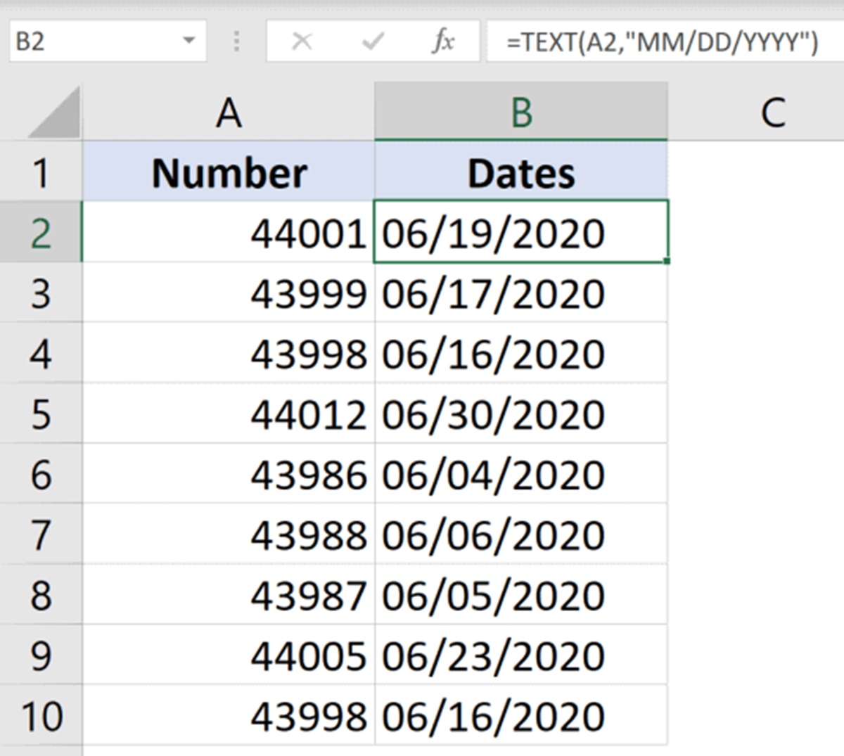
Using the TEXT function: The TEXT function in Excel is useful for converting a serial number into a specific date format. Utilize the formula “=TEXT(serial_number, “format”)” where “serial_number” is the cell containing the serial number and “format” is the desired date format. For example, to convert a serial number into the format “mmm-dd-yyyy”, use “=TEXT(A1, “mmm-dd-yyyy”)”.
Using the Paste Special function: If you have a column of serial numbers that you want to convert to dates, you can use the Paste Special function. Select the column with serial numbers, right-click, choose “Paste Special,” and select “Values.” Then, under “Operation,” choose “Add” to convert the serial numbers to dates.

By converting serial numbers to dates, you gain the ability to perform accurate date-related calculations, sorting, and filtering. This ensures that your data is correctly interpreted and analyzed within the context of time.

It is important to note that Excel stores dates as serial numbers based on the specific date system (e.g., the 1900 date system). Be mindful of any limitations or quirks associated with the date system you are using.

When dealing with large datasets, using Excel’s built-in functions or paste special techniques can save time and effort by automating the conversion process and ensuring the accuracy of the converted dates.

By converting serial numbers to dates, you can effectively work with and manipulate time-based data in Excel, providing valuable insights and facilitating better decision-making.

Adjusting the Date Format for Serial Numbers

In Excel, serial numbers are used to represent dates, but they may not always display in the desired date format. However, Excel provides various options to adjust the date format for serial numbers, allowing you to customize how dates are presented. Here’s how you can adjust the date format:

Select the cell or range of cells containing the serial number dates that you want to format.
Right-click on the selected cells and choose “Format Cells” from the context menu.
In the “Number” tab, select the “Date” category.
Select the desired date format from the options provided, such as “Short Date,” “Long Date,” or a specific custom format.
You can also customize the date format by clicking the “Custom” category and entering a specific format code.
Click “OK” to apply the formatting changes.

By adjusting the date format for serial numbers, you can control how dates are displayed based on your preferences or regional formatting conventions. This can include modifying the order of day, month, and year, specifying date separators, or adding additional details like the day of the week.

Excel offers a wide range of pre-defined date formats to choose from, catering to various regional preferences and specific formatting requirements. Additionally, you can create custom date formats using format codes to display dates in a format that best suits your needs.

Keep in mind that Excel’s date system, such as the 1900 date system, may have limitations or quirks in recognizing specific dates. Therefore, it is important to ensure that the date format accurately reflects the intended date representation and aligns with the date system being used in Excel.

By adjusting the date format for serial numbers, you can enhance the readability and presentation of dates in Excel, making it easier for yourself and others to interpret and work with time-related data.

Working with Dates and Serial Numbers in Excel Formulas and Functions

Excel provides a wide range of formulas and functions to perform calculations and manipulations on dates and serial numbers. These formulas and functions allow you to extract specific information from dates, perform arithmetic operations, calculate date differences, and more. Here are some commonly used formulas and functions:

DATEVALUE: This function converts a date string into a serial number. For example, “=DATEVALUE(“1/1/2022″)” will return the serial number representing January 1, 2022. This function is useful when working with dates in text format.
MONTH, DAY, YEAR: These functions extract the month, day, and year components from a given date or serial number. For instance, “=MONTH(A1)” will return the month component from the date stored in cell A1.
TODAY: This function displays the current date as a serial number. It is updated automatically each time the worksheet is reopened or recalculated. For example, “=TODAY()” will return the current date.
EDATE: This function calculates the date that is a specified number of months before or after a given date. It is useful for performing calculations involving month-based intervals. For instance, “=EDATE(A1, 6)” will return a date six months after the date in cell A1.
DATEDIF: This function calculates the difference between two dates in various date units (such as years, months, or days). For example, “=DATEDIF(A1, A2, “Y”)” will calculate the number of complete years between the dates in cells A1 and A2.
NETWORKDAYS: This function calculates the number of working days between two dates, excluding weekends and specified holidays. It is useful for tracking business days or calculating project durations. For example, “=NETWORKDAYS(A1, A2)” will calculate the number of working days between the dates in cells A1 and A2.

These formulas and functions, among many others in Excel, enable you to perform complex calculations and manipulations on dates and serial numbers easily. By leveraging these tools, you can analyze trends, track timelines, calculate durations, and gain valuable insights from your data.

Remember to ensure that the date formats and data types are compatible with the formulas and functions you are using. Invalid formats may result in errors or unexpected results.

Experimenting with different formulas and functions will help you unlock the full potential of dates and serial numbers in Excel, making your data analysis more efficient and precise.

Calculating the Difference Between Two Dates Using Serial Numbers

In Excel, you can use serial numbers to calculate the difference between two dates, enabling you to analyze durations, track timelines, or determine the gap between specific events. By performing arithmetic operations on serial numbers representing dates, you can obtain valuable insights from your data. Here are some methods to calculate the difference between two dates:

Subtraction: Subtracting one serial number from another gives you the difference in days between two dates. For example, if cell A1 contains the start date and cell B1 contains the end date, the formula “=B1 – A1” will return the number of days between the two dates.
DATEDIF Function: The DATEDIF function calculates the difference between two dates in various date units, such as years, months, or days. For example, “=DATEDIF(A1, B1, “Y”)” calculates the number of complete years between the dates in cells A1 and B1.
YEARFRAC Function: The YEARFRAC function calculates the difference between two dates in terms of a fraction of a year. It is useful when you need to determine a fractional difference between two dates. For example, “=YEARFRAC(A1, B1)” will return the fractional difference (in years) between the dates in cells A1 and B1.
NETWORKDAYS Function: The NETWORKDAYS function allows you to calculate the number of working days between two dates, excluding weekends and specified holidays. It is useful for tracking business days or project durations. For example, “=NETWORKDAYS(A1, B1)” will calculate the number of working days (excluding weekends) between the dates in cells A1 and B1.
Custom Formulas: You can create custom formulas to calculate the difference between two dates in a specific format or for a specific purpose. For instance, you can create a formula to calculate the difference in months, weeks, or any other custom unit of time.

When working with date differences, it’s important to ensure that the dates are properly formatted as serial numbers or recognized as date values. Otherwise, you may encounter unexpected results or errors in your calculations.

By calculating the difference between two dates using serial numbers, you can gain insights into the time duration between events or make informed decisions based on timelines and trends present in your data.

Sorting Data Based on Serial Numbers or Dates

Sorting data based on serial numbers or dates in Excel allows you to organize information in a logical sequence, making it easier to analyze and interpret. Excel provides powerful sorting capabilities that enable you to arrange data in ascending or descending order based on serial numbers or dates. Here’s how you can sort data using these criteria:

Normal Sorting: Select the range of data you want to sort. Open the “Data” tab in the Excel ribbon, click on the “Sort” button. In the “Sort” dialog box, choose the column that contains the serial numbers or dates you want to sort by. Specify whether you want the data to be sorted in ascending or descending order. Click “OK” to sort the data based on the selected criterion.
Custom Sorting: Excel allows you to define custom sorting rules or criteria. Select the range of data and open the “Data” tab. Click on the “Sort” button and then the “Sort Options” button in the “Sort” dialog box. In the “Sort Options” dialog box, you can specify additional criteria for sorting, such as sorting by multiple columns or sorting based on a custom list. Click “OK” to apply the custom sorting rules.
Sorting Tables: If you have your data in an Excel table, you can easily sort the data by selecting the column header and using the sorting buttons that appear. Click on the sorting button to sort the data in ascending or descending order based on the selected column.

Sorting data based on serial numbers or dates can be useful in various scenarios. For example, you can sort sales data by date to analyze trends over time or sort a list of tasks by their due dates to prioritize them effectively.

When sorting data, it’s important to ensure that the serial numbers or dates are formatted correctly in Excel. Improper formatting may lead to incorrect sorting results. Additionally, ensure that any related data in adjacent columns is selected as well to maintain data integrity.

By sorting data based on serial numbers or dates, you can quickly organize and arrange information in a meaningful sequence, allowing for better analysis, decision-making, and understanding of trends and patterns in your data.

Filtering Data Based on Serial Numbers or Dates

Filtering data based on serial numbers or dates in Excel allows you to narrow down your dataset and focus on specific records or a particular time period. Excel provides powerful filtering capabilities that enable you to display only the data that meets certain criteria related to serial numbers or dates. Here’s how you can filter data using these criteria:

AutoFilter: Select the range of data you want to filter. Open the “Data” tab in the Excel ribbon and click on the “Filter” button. Dropdown arrows will appear in the header of each column. Click on the dropdown arrow of the column containing the serial numbers or dates you want to filter. Select the desired date or serial number criteria to display only the matching records.
Advanced Filter: Advanced Filter provides more complex filtering options. Select the range of data you want to filter and open the “Data” tab. Click on “Advanced” in the “Sort & Filter” group. In the “Advanced Filter” dialog box, choose the range that includes both the source data and the criteria. Specify the criteria based on the serial numbers or dates, and choose whether to filter in place or copy the filtered data to a different location. Click “OK” to apply the advanced filter.
Filter by Date Range: You can filter data within a specific date range. Using the AutoFilter or Advanced Filter methods, select the column containing the dates. In the filter dropdown, select the “Date Filters” option and choose the desired filter, such as “Between,” “Before,” or “After.” Specify the date range or target date to filter the data accordingly.

Filtering data based on serial numbers or dates can be beneficial in various scenarios. For example, you can filter sales data to focus on a specific month or year, or filter a project management list to display tasks due within a certain timeframe.

Keep in mind that proper formatting of the serial numbers or dates is crucial for accurate filtering results. Ensure that the date values are formatted correctly and recognized as date data types in Excel.

By filtering data based on serial numbers or dates, you can quickly extract specific information from large datasets, analyze trends within a specific time period, or narrow down your focus to relevant records, thereby facilitating effective data analysis and decision-making.

Summary and Key Takeaways

In this article, we explored various aspects of working with serial numbers and dates in Excel. Let’s summarize the key takeaways:

– Serial numbers in Excel are consecutive numbers or identifiers used to establish a unique identity for records or items in a list or database.

– Serial numbers can be automatically generated using the Fill Handle, the ROW function, or the SEQUENCE function in Excel.

– Formatting options in Excel allow you to customize the appearance of serial numbers, including number formatting, decimal places, and adding prefixes or suffixes.

– Serial numbers in Excel represent dates, with each date assigned a unique numeric value that follows a sequential pattern.

– Dates can be displayed by formatting serial numbers, converting them to recognizable dates.

– Excel offers formulas and functions to perform calculations, extract information, and manipulate dates and serial numbers effectively.

– When working with dates, be mindful of Excel’s date system and any limitations associated with it, such as handling leap years.

– Sorting data based on serial numbers or dates helps organize information and make it easier to analyze and interpret.

– Filtering data based on serial numbers or dates allows you to narrow down the dataset and focus on specific records or time periods.

By mastering the concepts and techniques discussed in this article, you can efficiently work with serial numbers and dates in Excel. This will enhance your ability to manage data, perform calculations, and draw meaningful insights from your datasets.