
Overview of Small and Large Function
The Small and Large functions are powerful tools in Excel that allow users to quickly find the smallest or largest values in a given range. These functions are particularly useful when working with large sets of data and need to identify the minimum or maximum values.
The Small function returns the nth smallest value in a range, while the Large function returns the nth largest value. Both functions are useful for analyzing data and can be applied to various scenarios, such as finding the smallest sales amount or identifying the largest project budget.
The syntax for the Small function is:
SMALL(range, k)
Where range is the range of cells that you want to evaluate, and k is the position of the value you want to retrieve from the smallest to the largest. For example, to find the smallest value in a range A1:A10, you would use the formula:
=SMALL(A1:A10, 1)
This would return the smallest value in the range A1:A10.
On the other hand, the syntax for the Large function is:
LARGE(range, k)
The parameters range and k are similar to the Small function. For instance, to find the largest value in a range A1:A10, you would use the formula:
=LARGE(A1:A10, 1)
This would return the largest value in the range A1:A10.
Both the Small and Large functions can be combined with other Excel functions to perform more complex calculations. For instance, you can use them in conjunction with the IF function to apply specific conditions before retrieving the smallest or largest value.
In the following sections, we will explore practical examples of how to use the Small and Large functions to find the smallest and largest values, and demonstrate how they can be combined for more advanced analysis.
Syntax of Small Function
The Small function in Excel is a powerful tool that allows you to find the nth smallest value in a range. It is particularly useful when working with large sets of data and need to identify the minimum values.
The syntax for the Small function is:
SMALL(range, k)
Where:
- range: The range of cells that you want to evaluate.
- k: The position of the value you want to retrieve from the smallest to the largest.
For example, let’s say you have a range of values in cells A1 to A10, and you want to find the smallest value. You would use the Small function as follows:
=SMALL(A1:A10, 1)
This formula will return the smallest value in the range A1:A10 because we specified the position “1” as the second argument.
You can also retrieve other small values by changing the second argument. For example, if you want to find the second smallest value in the range, you would use:
=SMALL(A1:A10, 2)
This time, the formula will return the second smallest value in the range A1:A10.
It’s important to note that if you provide a value of “0” or a negative value for the second argument, the Small function will return an error. Also, if there are duplicate values in the range, the Small function will return the smallest value only once.
By combining the Small function with other Excel functions like IF, SUM, or AVERAGE, you can perform more complex calculations and analyze your data more effectively. This versatility makes the Small function a valuable tool for data analysis and decision-making.
Example 1: Using Small Function to Find Smallest Value
Let’s imagine you have a dataset that contains the sales figures of your company’s products for the past month. You want to find the product with the smallest sales amount. Here’s how you can use the Small function to accomplish this:
- Assume that the sales figures are listed in column B, starting from cell B2.
- Enter the formula
=SMALL(B2:B10, 1)in a different cell to find the smallest sales value. - The Small function will evaluate the range B2:B10 and return the smallest value in that range.
For example, let’s say the sales values are as follows:
| Product | Sales |
|---|---|
| Product A | 100 |
| Product B | 150 |
| Product C | 80 |
| Product D | 120 |
| Product E | 90 |
Applying the Small function to the range B2:B10, the formula =SMALL(B2:B10, 1) will return the smallest sales value, which is 80, corresponding to Product C.
This method allows you to easily find the product with the smallest sales amount without manually sorting the data or using other complex formulas.
By changing the second argument of the Small function, you can retrieve the second, third, or any other small value in the range. For instance, using =SMALL(B2:B10, 2) would return the second smallest value, which is 90.
Using the Small function simplifies the process of finding the smallest value in a dataset and allows you to perform quick and accurate analysis of your data.
Example 2: Using Small Function with Array Formula
The Small function can also be used with an array formula to handle multiple criteria and retrieve multiple smallest values at once. Let’s explore an example to understand how this can be done:
- Assume that you have a dataset containing the scores of students in different subjects. The data is organized with student names in column A, subjects in row 1, and scores in corresponding cells.
- You want to find the three smallest scores for each subject. Here’s how you can achieve this using the Small function with an array formula:
- Select a range of cells where you want the results to be displayed. For instance, you can select cells D2:F4.
- Enter the array formula
=SMALL($B$2:$D$10, ROW($1:$3))in cell D2. - Press
Ctrl + Shift + Enterto apply the array formula. - The array formula will calculate the smallest values of each row in the range B2:D10.
For example, let’s assume the scores are as follows:
| Student | Math | Science | English |
|---|---|---|---|
| John | 80 | 70 | 75 |
| Emily | 90 | 85 | 80 |
| Michael | 85 | 75 | 85 |
Applying the array formula =SMALL($B$2:$D$10, ROW($1:$3)), you will obtain the three smallest scores for each subject. The result will be displayed in cells D2:F4:
| Math | Science | English |
|---|---|---|
| 80 | 70 | 75 |
| 85 | 75 | 80 |
| 90 | 85 | 85 |
By using the Small function with an array formula, you can efficiently retrieve multiple smallest values for each subject. This technique is helpful in analyzing large datasets and identifying the students with the lowest scores across different subjects.
Syntax of Large Function
The Large function in Excel allows you to find the nth largest value in a range. It is particularly useful when you need to identify the maximum values in a dataset or perform data analysis tasks.
The syntax for the Large function is:
LARGE(range, k)
Where:
- range: The range of cells that you want to evaluate.
- k: The position of the value you want to retrieve from the largest to the smallest.
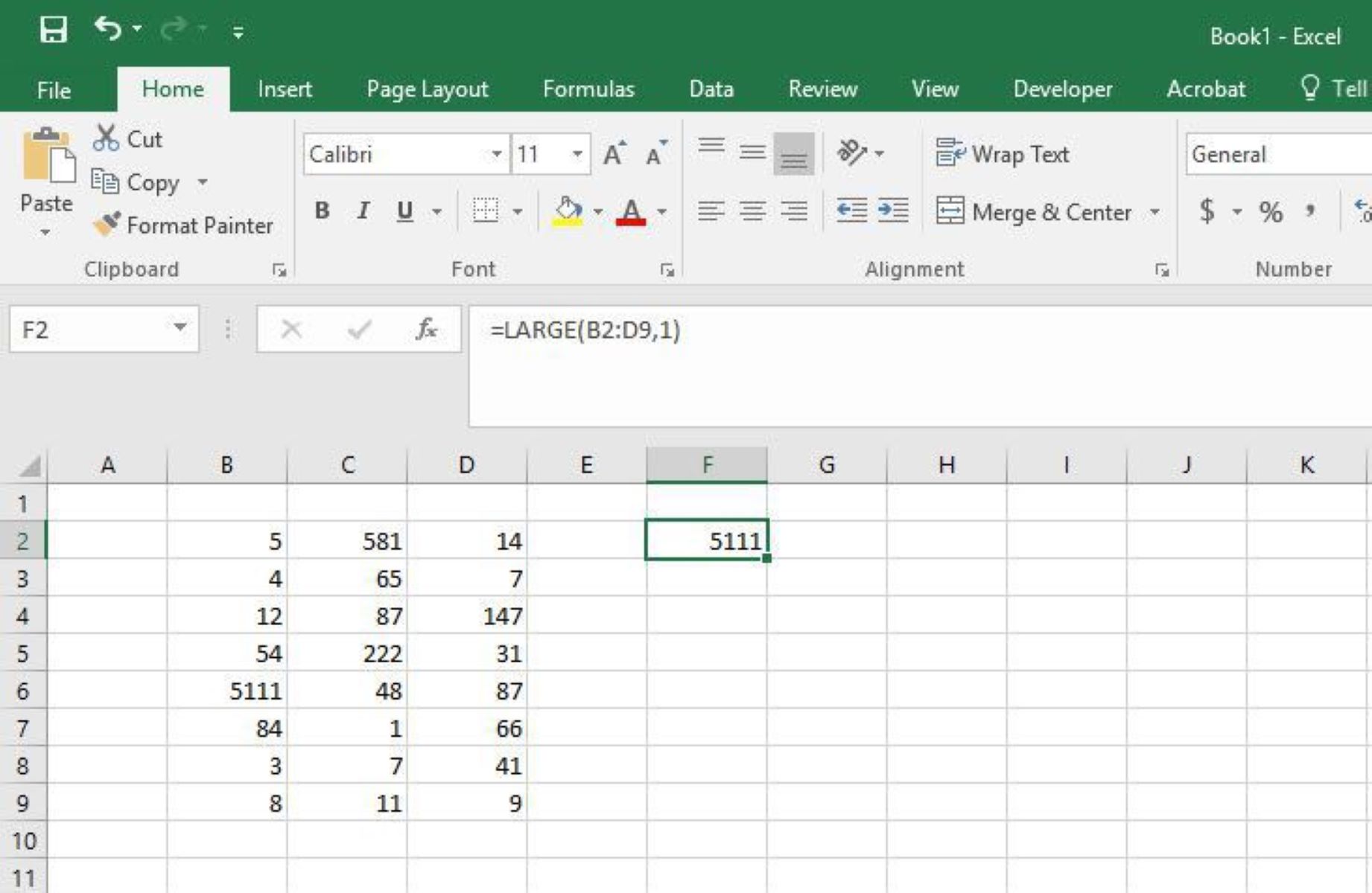
For example, suppose you have a range of values in cells A1 to A10 and you want to find the largest value. You can use the Large function as follows:
=LARGE(A1:A10, 1)
This formula will return the largest value in the range A1:A10 because we specified the position “1” as the second argument.
Similarly to the Small function, you can retrieve other large values by changing the second argument. For example, if you want to find the second largest value in the range, you would use:
=LARGE(A1:A10, 2)
By providing the value “2” as the second argument, the formula will return the second largest value in the range A1:A10.
It’s important to note that if you provide a value of “0” or a negative value for the second argument, the Large function will return an error. Additionally, if there are duplicate values in the range, the Large function will return the largest value only once.
Just like the Small function, the Large function can be combined with other Excel functions to perform more complex calculations and gain deeper insights from your data. This versatility makes the Large function a valuable tool for data analysis and decision-making in Excel.
Example 3: Using Large Function to Find Largest Value
Let’s say you have a dataset that contains the daily temperatures recorded in a city for the past month. You want to find the day with the highest temperature. Here’s how you can use the Large function to accomplish this:
- Assume that the temperature readings are listed in column B, starting from cell B2.
- Enter the formula
=LARGE(B2:B32, 1)in a different cell to find the largest temperature value. - The Large function will evaluate the range B2:B32 and return the largest value in that range.
For example, let’s assume the temperature readings are as follows:
| Date | Temperature (°C) |
|---|---|
| 1st July | 30 |
| 2nd July | 32 |
| 3rd July | 29 |
| 4th July | 35 |
| 5th July | 31 |
Applying the Large function to the range B2:B32, the formula =LARGE(B2:B32, 1) will return the largest temperature value, which is 35, corresponding to the 4th of July.
This method allows you to easily find the day with the highest temperature without manually sorting the data or using other complex formulas.
By changing the second argument of the Large function, you can retrieve the second, third, or any other large value in the range. For instance, using =LARGE(B2:B32, 2) would return the second largest value, which is 32.
The Large function simplifies the process of finding the largest value in a dataset and allows you to perform quick and accurate analysis of your data, making it a valuable tool for analyzing temperatures, sales figures, stock prices, and various other types of data.
Example 4: Using Large Function with Array Formula
The Large function can be combined with an array formula in Excel to find multiple largest values based on specific criteria. Let’s explore an example to understand how this can be done:
- Assume you have a dataset of student scores in different subjects. The data is organized with student names in column A, subjects in row 1, and scores in the corresponding cells.
- You want to find the three highest scores for each subject. Here’s how you can achieve this using the Large function with an array formula:
- Select a range of cells where you want the results to be displayed. For instance, you can select cells D2:F4.
- Enter the array formula
=LARGE($B$2:$D$10, ROW($1:$3))in cell D2. - Press
Ctrl + Shift + Enterto apply the array formula. - The array formula will calculate the largest values from each row in the range B2:D10.
For example, let’s assume the scores are as follows:
| Student | Math | Science | English |
|---|---|---|---|
| John | 80 | 70 | 75 |
| Emily | 90 | 85 | 80 |
| Michael | 85 | 75 | 85 |
Applying the array formula =LARGE($B$2:$D$10, ROW($1:$3)), you will obtain the three largest scores for each subject. The result will be displayed in cells D2:F4:
| Math | Science | English |
|---|---|---|
| 90 | 85 | 85 |
| 85 | 80 | 80 |
| 80 | 75 | 75 |
By using the Large function with an array formula, you can efficiently retrieve multiple largest values for each subject. This allows you to analyze student scores, identify top performers, and gain insights from your data.
Combining Small and Large Functions for Advanced Analysis
Excel’s Small and Large functions are powerful on their own, but they become even more valuable when combined to perform advanced data analysis. By using these functions together, you can extract specific data points, identify outliers, and gain deeper insights from your datasets.
One common application of combining the Small and Large functions is to analyze the distribution of values within a dataset. By finding the smallest and largest values, you can determine the range and spread of the data. For example, you can calculate the difference between the largest and smallest values to understand the variation or use percentiles to divide the dataset into groups.
Another use case is to find the second smallest or second largest value in a range. This can be achieved by nesting the Small or Large function within another Small or Large function. For instance, to find the second smallest value, you can use =SMALL(A1:A10, 2) to retrieve the smallest value, and then wrap it in another Small function: =SMALL(A1:A10, SMALL(IF(A1:A10<>SMALL(A1:A10, 1), ROW(A1:A10)), 1)).
By combining Small and Large with other Excel functions like IF, SUM, AVERAGE, or INDEX, you can perform complex calculations and make more advanced analyses of your data. For example, you can use these functions to find the average of the largest values, sum the smallest values that meet certain criteria, or retrieve the corresponding values from another column based on the ranking.
Whether you need to analyze sales figures, student scores, or any other dataset, combining Small and Large functions allows you to dive deeper into the data and uncover valuable insights. By exploring different combinations and adapting them to specific analysis scenarios, you can make more informed decisions and enhance your data-driven decision-making process.
Example 5: Finding Second Smallest Value using Small and Large Functions
Let’s say you have a dataset that contains the monthly expenses of a business for the past year. You want to find the second smallest expense value. Here’s how you can use the Small and Large functions together to accomplish this:
- Assume that the monthly expenses are listed in column B, starting from cell B2.
- Enter the formula
=SMALL(B2:B13, 2)in a different cell to find the second smallest expense value. - The Small function will evaluate the range B2:B13 and return the second smallest value in that range.
For example, let’s assume the monthly expenses are as follows:
| Month | Expense ($) |
|---|---|
| January | 1000 |
| February | 1500 |
| March | 1200 |
| April | 900 |
| May | 1100 |
Applying the formula =SMALL(B2:B13, 2), the function will return the second smallest expense value, which is 1000. This corresponds to the month of January.
By combining the Small and Large functions in this way, you can easily find the value that ranks at any position in a range. Changing the second argument of the Small function allows you to retrieve the third smallest value, fourth smallest value, and so on.
This method is particularly useful for analyzing expenses, sales figures, or any other dataset where you need to identify values beyond the lowest or highest values. By using both Small and Large functions together, you can perform more advanced analysis and gain better insights from your data.
Example 6: Finding Second Largest Value using Small and Large Functions
Suppose you have a dataset that contains the quarterly revenue of a company over the past few years. You want to find the second-largest revenue value. Here’s how you can use the Small and Large functions together to accomplish this:
- Assume that the revenue data is listed in column B, starting from cell B2.
- Enter the formula
=LARGE(B2:B20, 2)in a different cell to find the second-largest revenue value. - The Large function will evaluate the range B2:B20 and return the second-largest value in that range.
For example, let’s assume the quarterly revenue values are as follows:
| Quarter | Revenue ($) |
|---|---|
| Q1 2018 | 500,000 |
| Q2 2018 | 600,000 |
| Q3 2018 | 450,000 |
| Q4 2018 | 550,000 |
| Q1 2019 | 700,000 |
Applying the formula =LARGE(B2:B20, 2), the function will return the second-largest revenue value, which is $600,000. This corresponds to the revenue in Q2 of 2018.
By using the Small and Large functions together, you can easily find the value that ranks at any position in a range. Likewise, changing the second argument of the Large function allows you to retrieve the third-largest value, fourth-largest value, and so on.
This approach is especially useful for financial analysis, sales tracking, or any other dataset where you need to identify values beyond the smallest or largest values. By leveraging both the Small and Large functions, you can perform more advanced analysis and gain deeper insights from your data.