
Overview of the COUNTIF Function
The COUNTIF function in Excel allows you to count the number of cells within a range that meet specific criteria. It is a powerful tool that can be used to analyze data and obtain valuable insights. Whether you are working with numerical values, text, or even dates and times, the COUNTIF function can efficiently count cells that match your specified conditions.
The basic syntax of the COUNTIF function is:
=COUNTIF(range, criteria)
The “range” parameter represents the range of cells you want to evaluate, while the “criteria” parameter defines the condition or criteria that must be met for a cell to be counted. The criteria can be a number, a text value, a logical expression, or a cell reference containing any of these.
One of the key benefits of using the COUNTIF function is its flexibility. You can perform simple count operations by specifying a single criteria, or you can use multiple criteria to make your analysis more specific. Additionally, the COUNTIF function supports the use of wildcards, logical operators, cell references, and even formulas, allowing for greater customization.
By using the COUNTIF function, you can quickly answer questions such as:
- How many sales transactions exceeded a specific amount?
- How many employees have a performance rating of “excellent”?
- How many customers have made a purchase within the last month?
Counting cells based on certain criteria can help you better understand your data, identify trends, and make informed decisions. Whether you are working on a complex analysis or simply need to get a quick count, the COUNTIF function is a valuable tool to have in your Excel arsenal.
As we delve deeper into the COUNTIF function, we will explore various examples and scenarios to help you master its usage and unlock its full potential.
Syntax of the COUNTIF Function
The syntax of the COUNTIF function in Excel is straightforward and easy to understand. It follows the format:
=COUNTIF(range, criteria)
The “range” parameter represents the range of cells that you want to evaluate for the specified criteria. This can be a single column, multiple columns, or even an entire worksheet. It is important to note that the COUNTIF function only counts cells within the specified range that meet the criteria.
The “criteria” parameter defines the condition or criteria that a cell must meet in order to be counted. The criteria can be a number, a text value, a logical expression, or even a cell reference containing any of these. For example, you can use criteria such as “>10” to count cells that are greater than 10, or “Red” to count cells that contain the word “Red”.
It is important to enclose text criteria in quotation marks (“”) to ensure that Excel recognizes them as strings. If you are using a cell reference as your criteria, no quotation marks are necessary as Excel will automatically interpret it as a reference.
Let’s take a look at a few examples to better understand the syntax of the COUNTIF function:
=COUNTIF(A2:A10, ">5"): This formula counts the number of cells in the range A2 to A10 that are greater than 5.=COUNTIF(B2:B10, "Red"): This formula counts the number of cells in the range B2 to B10 that contain the word “Red”.=COUNTIF(C2:C10, D2): This formula counts the number of cells in the range C2 to C10 that match the value in cell D2.
By understanding the syntax of the COUNTIF function, you can easily customize your formulas to suit your specific requirements. Whether you are performing simple counts or complex analyses, the COUNTIF function provides you with the flexibility to efficiently count cells based on your chosen criteria.
Now that we have covered the syntax of the COUNTIF function, let’s explore its usage in more detail to unleash its full potential in Excel.
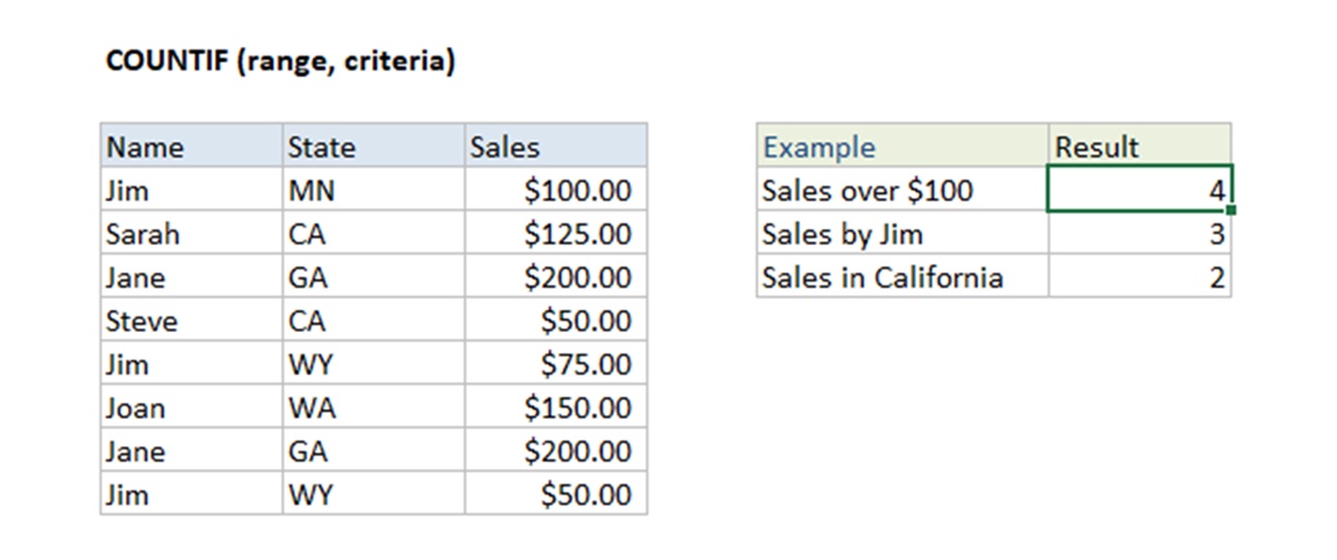
Using the COUNTIF Function with a Single Criteria
The COUNTIF function in Excel allows you to count the number of cells within a range that meet a single specified criteria. This provides you with a powerful tool for analyzing and summarizing data based on a specific condition.
To use the COUNTIF function with a single criteria, you simply need to specify the range of cells you want to evaluate and the criteria itself. The syntax for this operation is:
=COUNTIF(range, criteria)
Here’s an example to illustrate how you can use the COUNTIF function with a single criteria:
Let’s say you have a dataset of test scores for a class of students in column A, and you want to count the number of students who scored above 80. You can use the following formula:
=COUNTIF(A2:A10, ">80")
In this example, the range is specified as A2:A10, which encompasses the test score values for the students. The criteria “>80” means that only the scores greater than 80 will be counted. The function will return the total count of all the cells that meet this condition.
The same principle applies for any type of criteria you want to use. Whether you are counting cells that contain specific words, dates, or numbers within a range, the COUNTIF function can handle it all. You have the flexibility to count cells that match the criteria exactly or cells that meet a certain range of values.
By using the COUNTIF function with a single criteria, you can quickly and efficiently obtain valuable information from your dataset. It allows you to identify patterns, trends, and specific occurrences that meet your desired condition.
As you become more familiar with using the COUNTIF function, you’ll realize its versatility and how it can be applied across various scenarios to perform meaningful calculations with ease.
Using the COUNTIF Function with Multiple Criteria
The COUNTIF function in Excel not only allows you to count cells based on a single criteria, but it also enables you to count cells that meet multiple criteria simultaneously. This is a powerful feature that provides you with enhanced flexibility and the ability to perform more complex analyses.
When using the COUNTIF function with multiple criteria, you need to employ the concept of logical operators, such as AND and OR, to define the conditions that must be met. The syntax for using multiple criteria with the COUNTIF function is:
=COUNTIFS(criteria_range1, criteria1, criteria_range2, criteria2, ...)
Let’s take an example to illustrate how you can use the COUNTIF function with multiple criteria:
Suppose you have a sales dataset with columns for “Product,” “Region,” and “Sales.” You want to count the number of products sold in the “North” region with sales above $500. You can use the following formula:
=COUNTIFS(B2:B10, "North", C2:C10, ">500")
In this example, we have used two sets of criteria. The first set (B2:B10, "North") specifies that we want to count cells where the “Region” column is equal to “North”. The second set (C2:C10, ">500") states that we want to count cells where the “Sales” column is greater than $500.
The COUNTIF function evaluates both sets of criteria simultaneously and returns the count of cells that meet all the conditions specified.
You can include as many sets of criteria as needed, each consisting of a criteria range and a criteria value. Excel will count only the cells that meet all the specified conditions.
Using the COUNTIF function with multiple criteria allows you to perform more detailed data analysis by combining different conditions. It provides you with the ability to count cells that meet complex combinations of criteria, giving you greater insight into your data.
By understanding and effectively utilizing the COUNTIF function with multiple criteria, you gain the power to perform intricate calculations and extract meaningful information from your datasets.
Using Wildcards in the COUNTIF Function
The COUNTIF function in Excel allows you to use wildcard characters to count cells that match a pattern or contain specific text. Wildcards are special characters that represent unknown or variable characters within a value. This feature provides you with greater flexibility in searching for and counting cells with specific patterns or partial matches.
Excel supports two wildcard characters: the asterisk (*) and the question mark (?). Here’s how you can use them:
- The asterisk (*) represents any number of characters or a string of text. For example, the criteria “A*” would count all cells that begin with the letter A.
- The question mark (?) represents any single character. For example, the criteria “?at” would count cells that have any single character followed by “at”.
Let’s explore a few examples to understand how to use wildcards in the COUNTIF function:
Suppose you have a dataset with a list of names in column A, and you want to count the number of names that begin with the letter “J”. You can use the following formula:
=COUNTIF(A2:A10, "J*")
In this example, the criteria “J*” counts all cells that start with the letter “J”. The asterisk (*) represents any number of characters that follow the letter “J”.
Similarly, you can use the question mark (?) wildcard to perform more specific searches. Let’s say you have a dataset with a list of email addresses, and you want to count the number of email addresses that end with “.com”. You can use the following formula:
=COUNTIF(A2:A10, "*@*.com")
In this example, the criteria “*@*.com” counts all cells that have an “@” symbol followed by any number of characters, then a dot (.), and finally the letters “com”.
By using wildcards in the COUNTIF function, you can create dynamic and flexible criteria to count cells that match specific patterns or contain certain text. This allows you to perform more advanced searches and obtain more precise counts based on your specific requirements.
Experiment with different wildcard combinations to explore the possibilities and unlock the full potential of the COUNTIF function in Excel.
Using the COUNTIF Function with Dates and Times
The COUNTIF function in Excel can be highly valuable when working with dates and times. It allows you to count cells that meet specific criteria based on their date or time values. Whether you need to count the number of cells that fall within a certain date range, meet a specific date condition, or satisfy a time constraint, the COUNTIF function can handle it all.
When using the COUNTIF function with dates and times, it is important to ensure that your criteria are formatted correctly to match the format of the values in the cells you are evaluating. Here are a few examples to illustrate how to use the COUNTIF function with dates and times:
Counting cells in a date range:
Let’s say you have a dataset with a list of project deadlines in column A, and you want to count the number of deadlines that fall within a specific date range. You can use the following formula:
=COUNTIF(A2:A10,">=2022-01-01")
In this example, the criteria “>=2022-01-01” counts all cells that have a date value greater than or equal to January 1, 2022. The COUNTIF function will evaluate the dates in the range and return the count of cells that meet this condition.
Counting cells with a specific date:
If you want to count cells that have a specific date, you can use the following formula:
=COUNTIF(A2:A10,"2022-02-14")
In this example, the criteria “2022-02-14” counts all cells that have the date February 14, 2022. The COUNTIF function will search for exact matches and provide the count accordingly.
Counting cells within a specific time range:
Suppose you have a dataset with a list of appointment times in column A, and you want to count the number of appointments that fall within a specific time range. You can use the following formula:
=COUNTIF(A2:A10,">=9:00 AM", A2:A10,"<=12:00 PM")
In this example, the criteria use logical operators to count all cells that have a time value greater than or equal to 9:00 AM and less than or equal to 12:00 PM. The COUNTIF function will evaluate the appointment times and return the count of cells that satisfy both conditions.
Using the COUNTIF function with dates and times allows you to perform various analyses and obtain valuable insights from your dataset. By accurately defining your criteria and leveraging the power of the COUNTIF function, you can efficiently count cells based on your specific date and time requirements.
Using the COUNTIF Function with Text
The COUNTIF function in Excel is not only useful for numerical and date/time values, but it is also a versatile tool for working with text data. You can use the COUNTIF function to count cells that match specific text criteria, allowing for effective analysis and summarization of your dataset.
When using the COUNTIF function with text, you can specify the criteria as a string of text, case-sensitive words, or even partial matches using wildcards. Here are a few examples to illustrate how to use the COUNTIF function with text:
Counting cells that match specific text criteria:
Suppose you have a dataset with a list of job titles in column A, and you want to count the number of cells that contain the word "Manager". You can use the following formula:
=COUNTIF(A2:A10, "Manager")
In this example, the criteria "Manager" counts all cells that contain the exact word "Manager". The COUNTIF function will evaluate the cells in the range and provide the count of cells that meet this condition.
Counting cells that match case-sensitive text:
If you need to perform a case-sensitive count, you can modify the formula using the EXACT function. Let's say you have a dataset with employee names in column A, and you want to count the number of cells that contain the name "John" in uppercase. You can use the following formula:
=COUNTIF(A2:A10, "=EXACT("John",A2:A10)")
In this example, the EXACT function within the COUNTIF criteria compares the exact text match between "John" and the cells in the range. The COUNTIF function will return the count of cells that contain the name "John" in uppercase.
Counting cells with partial text matches using wildcards:
If you want to count cells with partial text matches, you can utilize wildcard characters. For example, let's say you have a dataset with product names in column A, and you want to count the number of cells that start with the letter "S". You can use the following formula:
=COUNTIF(A2:A10, "S*")
In this example, the criteria "S*" counts all cells that begin with the letter "S". The asterisk (*) serves as a wildcard character representing any number of characters that follow the letter "S".
Using the COUNTIF function with text criteria allows you to efficiently count cells based on specific text conditions. Whether you need to count exact matches, case-sensitive matches, or partial matches, the COUNTIF function provides you with the flexibility to perform accurate text analysis within your datasets.
Using the COUNTIF Function with Logical Operators
The COUNTIF function in Excel allows you to use logical operators, such as greater than (>), less than (<), equal to (=), not equal to (<>, or !=), and more, to define specific criteria for counting cells. By utilizing logical operators, you can perform more advanced analysis and obtain counts based on complex conditions.
Here are a few examples to demonstrate how to use logical operators with the COUNTIF function:
Counting cells greater than a specific value:
Suppose you have a dataset with exam scores in column A, and you want to count the number of cells that have scores greater than 80. You can use the following formula:
=COUNTIF(A2:A10, ">80")
In this example, the criteria ">80" counts all cells that have scores greater than 80. The COUNTIF function will evaluate the values in the range and provide the count of cells that meet this condition.
Counting cells that are not equal to a specific value:
If you need to count cells that are not equal to a certain value, you can use the not equal to operator (<>, or !=). Let's say you have a dataset with student grades in column A, and you want to count the number of cells that have grades other than "A". You can use the following formula:
=COUNTIF(A2:A10, "<>A")
In this example, the criteria "<>A" counts all cells that are not equal to "A". The COUNTIF function will evaluate the values in the range and return the count of cells that do not match this condition.
Counting cells that meet multiple conditions using logical operators:
You can also combine logical operators to count cells that meet multiple conditions simultaneously. For instance, suppose you have a dataset with sales data in column A and you want to count the number of cells that have sales greater than 500 and occurred in the month of January. You can use the following formula:
=COUNTIFS(A2:A10, ">500", B2:B10, "January")
In this example, the first criteria ">500" counts cells with sales greater than 500, and the second criteria "January" counts cells that have the month "January". The COUNTIFS function compares both conditions for each corresponding cell and returns the count of cells that satisfy both conditions.
Utilizing logical operators with the COUNTIF function enables you to perform more complex analysis and obtain counts based on specific conditions. Whether you need to compare values, find cells that are not equal to a specific value, or evaluate multiple conditions, the COUNTIF function provides you with the necessary flexibility to meet your requirements.
Using the COUNTIF Function with Cell References
The COUNTIF function in Excel allows you to use cell references as criteria, making your formulas dynamic and adaptable. By referencing cells, you can create formulas that automatically update and adjust based on the values in those cells. This provides you with a powerful tool for analyzing and counting cells based on changing criteria or user inputs.
Let's explore how to use cell references with the COUNTIF function:
Referencing a cell for criteria:
Suppose you have a dataset with transaction amounts in column A, and you want to count the number of cells that exceed a certain threshold value specified in cell B1. You can use the following formula:
=COUNTIF(A2:A10, ">"&B1)
In this example, the criteria ">"&B1 combines the greater than operator (>) with the value in cell B1. The COUNTIF function will evaluate the values in the range A2:A10 and count the number of cells that meet the condition specified in cell B1.
Referencing cells for range and criteria:
You can also reference both the range and the criteria cells to make your formula more dynamic. Let's say you have sales data in column A, and you want to count the number of cells that meet a specific sales target mentioned in cell B1. The sales data starts from row 2 and goes down to row 10. You can use the following formula:
=COUNTIF(A2:A10, ">"&B1)
In this example, the range A2:A10 represents the range of cells to evaluate, and the criteria ">"&B1 combines the greater than operator (>) with the value in cell B1. The COUNTIF function will dynamically count the number of cells in the range A2:A10 that exceed the sales target specified in cell B1.
Using cell references with the COUNTIF function allows you to create formulas that can adapt to changing criteria or input values. By referencing cells, you can efficiently analyze and count cells based on dynamic conditions, making your analysis more flexible and robust.
Using the COUNTIF Function with Dynamic Ranges
The COUNTIF function in Excel can be utilized with dynamic ranges, allowing you to automatically adjust the range in your formulas as your data changes or expands. This feature is particularly useful when dealing with datasets that are constantly growing or when you want to create formulas that adapt to new data entries.
There are a few ways to use dynamic ranges with the COUNTIF function:
Using the OFFSET function:
The OFFSET function can be employed to create a dynamic range for the COUNTIF function. The OFFSET function returns a range that is a specified number of rows and columns from a starting point.
For instance, let's say you have a dataset with product sales in column A, and you want to count the number of cells that exceed a certain sales threshold. You can create a dynamic range using the OFFSET function to adjust the range as new sales entries are added:
=COUNTIF(OFFSET(A2, 0, 0, COUNTA(A:A)-1, 1), ">500")
In this example, the OFFSET function begins at cell A2 and creates a range that extends down to the last non-empty cell in column A (COUNTA(A:A)-1). The COUNTIF function is then applied to this dynamic range to count the number of cells that exceed the sales threshold of 500.
Using the INDEX function:
The INDEX function can also be utilized to create dynamic ranges. The function returns a reference to a specific cell or range of cells based on specified row and column numbers.
For example, let's say you have a dataset with customer ratings in column B, and you want to count the number of cells that have a rating of "5" or higher. You can create a dynamic range using the INDEX function as follows:
=COUNTIF(INDEX(B:B, 2):INDEX(B:B, COUNTA(B:B)), ">=5")
In this example, the INDEX function creates a range that starts from the second row (INDEX(B:B, 2)) and extends down to the last non-empty cell in column B (INDEX(B:B, COUNTA(B:B))). The COUNTIF function is then used to count the number of cells within this dynamic range that have a rating of 5 or higher.
By utilizing dynamic ranges with the COUNTIF function, you can create formulas that automatically adjust to changes in your data. This flexibility allows you to handle expanding datasets and ensure accurate counting even as new entries are added.
Using the COUNTIF Function with Formulas
The COUNTIF function in Excel can be combined with other formulas to perform more intricate and complex counting operations. This allows you to leverage the power of Excel's built-in functions and operators to create dynamic and customized counting solutions.
Here are a few examples of how you can use the COUNTIF function with formulas:
Using COUNTIF with arithmetic formulas:
You can incorporate arithmetic formulas within the COUNTIF function to count cells that meet certain mathematical conditions. For instance, let's say you have a dataset with quantities in column A, and you want to count the number of cells that have a quantity greater than the average quantity. You can use the following formula:
=COUNTIF(A2:A10, ">"&AVERAGE(A2:A10))
In this example, the AVERAGE function calculates the average of the range A2:A10, and the ">" operator compares each cell in the range to the average. The COUNTIF function then counts the number of cells that meet this condition.
Using COUNTIF with logical formulas:
You can combine logical formulas with the COUNTIF function to count cells that meet specific logical conditions. For example, let's say you have a dataset with customer ratings in column B, and you want to count the number of cells that have a rating of either "Excellent" or "Good". You can use the following formula:
=COUNTIF(B2:B10, "Excellent")+COUNTIF(B2:B10, "Good")
In this example, two COUNTIF functions are used, each targeting a specific rating. The results of both COUNTIF functions are then added together to obtain the total count of cells that meet either condition.
Using COUNTIF with text concatenation:
You can concatenate text values with other criteria within the COUNTIF function to count cells that meet specific text combination conditions. For instance, let's say you have a dataset with product codes in column C, and you want to count the number of cells where the product code starts with "ABC" and ends with "XYZ". You can use the following formula:
=COUNTIF(C2:C10, "ABC"&"*"&"XYZ")
In this example, the text values "ABC", "*", and "XYZ" are concatenated together to create the desired criteria. The COUNTIF function then counts the number of cells in the range C2:C10 that meet this combined condition.
By using the COUNTIF function with formulas, you can extend its functionality and perform advanced counting operations based on a wide range of conditions. This flexibility allows you to tailor your counting solutions according to your specific needs and deliver more comprehensive data analysis in Excel.
Common Errors and Troubleshooting Tips
While using the COUNTIF function in Excel, it's important to be aware of common errors that may occur and know how to troubleshoot them. Here are some common issues you may encounter and tips to resolve them:
Error: #VALUE!
This error occurs when the criteria argument in the COUNTIF function is not formatted correctly. To troubleshoot, check if the criteria are enclosed in quotation marks ("") for text values or if the syntax is correct for numerical or date/time values. Also, ensure that any cell references used as criteria are valid.
Error: #REF!
This error indicates that the range argument in the COUNTIF function refers to a cell or range that has been deleted or moved. To fix this error, update the range reference to include the correct cells that you want to count. Check if any rows or columns have been accidentally deleted or inserted, causing the references to be incorrect.
Error: #NAME?
This error occurs when Excel cannot recognize the function name. Double-check the spelling of the COUNTIF function and ensure that it is written correctly. If you are using a non-English version of Excel, the function might have a different name, so consult Excel's function library or documentation to find the appropriate function name.
Counting text values that contain wildcards
When using wildcards in the criteria argument, it's important to note that certain characters, such as asterisks (*) and question marks (?), have special meanings in Excel's pattern matching. If you want to count cells that contain these wildcard characters as part of their text values, you need to use the tilde (~) character as an escape character. For example, to count cells that contain the text "abc*xyz", use the criteria "abc~*xyz".
Updating the COUNTIF formula with new data
If you have a dynamic dataset where new data is added regularly, you may need to update your COUNTIF formula to include the new data. Consider using dynamic ranges, such as the OFFSET function or named ranges, to create formulas that automatically adjust as new data entries are added or removed.
By being aware of these common errors and utilizing troubleshooting tips, you can effectively identify and resolve issues that may arise when using the COUNTIF function in Excel. This will help ensure accurate counting and dependable functionality of your formulas.
Additional Tips and Tricks
When working with the COUNTIF function in Excel, there are several tips and tricks that can help you maximize its efficiency and usefulness. Here are some additional tips to enhance your counting capabilities:
Using named ranges:
Consider using named ranges to make your formulas more readable and easier to manage. By assigning a name to a specific range of cells, you can refer to the named range in your COUNTIF formula instead of specifying the cell references directly. Named ranges also automatically adjust when new data is added, ensuring your formulas remain accurate.
Combining COUNTIF with other functions:
Explore the possibilities of combining the COUNTIF function with other Excel functions to perform more advanced calculations. For example, you can use the SUM function in conjunction with COUNTIF to calculate the total sum of values that meet specific criteria.
Using data validation:
Implement data validation to ensure that the data entered into your worksheet meets specific criteria. By setting up data validation rules, you can control the types of data that can be entered, minimizing potential errors and ensuring accurate counting with the COUNTIF function.
Utilizing conditional formatting:
Apply conditional formatting to highlight cells that meet specific criteria. This visual representation can help you quickly identify and count cells based on different conditions. The COUNTIF function can be used in conjunction with conditional formatting formulas to create dynamic and visually appealing spreadsheets.
Using absolute and relative cell references:
When using cell references in your COUNTIF formula, determine whether you want the reference to be fixed (absolute) or adjust as the formula is copied to different cells (relative). Absolute references are denoted by the dollar sign ($) and can be useful when you want to fix the range or criteria to a specific cell while copying the formula.
Testing your formulas:
Always test your COUNTIF formulas with sample data to ensure they are providing the expected results. By doing so, you can identify any errors or discrepancies and make necessary adjustments before applying the formula to your actual dataset.
Exploring COUNTIFS and COUNTA functions:
In addition to COUNTIF, consider exploring the COUNTIFS and COUNTA functions. COUNTIFS allows you to count cells based on multiple criteria, while COUNTA counts the number of non-empty cells in a specified range. These functions can broaden your counting capabilities and provide more comprehensive analysis of your data.
By implementing these additional tips and tricks, you can enhance your use of the COUNTIF function and optimize your data analysis in Excel. Experiment with different techniques to find the best approach that suits your specific counting requirements.