
What is a Dynamic Range in Excel
In Excel, a dynamic range refers to a cell range that can automatically adjust its size based on the data it contains. Unlike a static range that has fixed start and end points, a dynamic range expands or shrinks as new data is added or removed from the spreadsheet.
Dynamic ranges are incredibly useful when working with data sets that may change in size over time. They allow you to perform calculations and analyze data without the need to manually update the range references each time new data is added.
Excel offers several methods to create dynamic ranges, including using functions like OFFSET, INDEX, or the combination of COUNT and OFFSET. One popular approach for creating dynamic ranges involves using the COUNTIF function in conjunction with the INDIRECT function.
By harnessing the power of these functions, you can create a dynamic range that will automatically adapt as new data is added or removed from your spreadsheet.
Dynamic ranges are commonly used in various Excel tasks, such as creating charts, performing calculations, applying conditional formatting, and more. They save time and effort by eliminating the need to manually update range references, ensuring that your formulas and functions always consider the most up-to-date data.
Furthermore, dynamic ranges help improve the efficiency and accuracy of your spreadsheet by reducing the likelihood of errors when adding or removing data. They provide flexibility and convenience, making it easier to handle fluctuating datasets and maintain the integrity of your calculations.
Now that we understand what a dynamic range is and its significance, let’s explore the COUNTIF function and the INDIRECT function in Excel, which are essential tools for creating dynamic ranges.
The COUNTIF Function in Excel
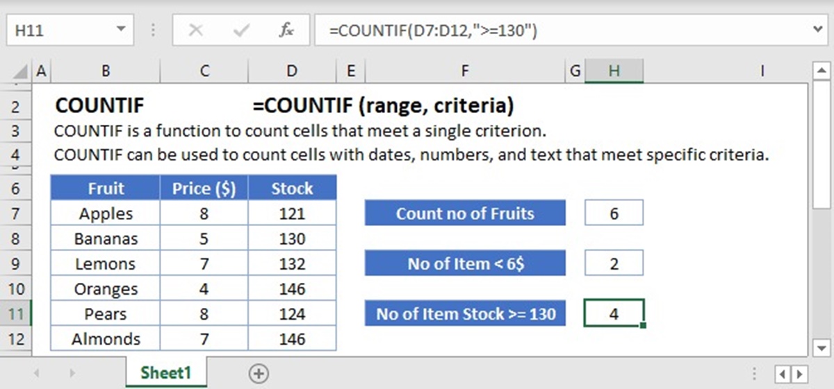
The COUNTIF function in Excel is a powerful tool that allows you to count the number of cells within a range that meet specific criteria. It is particularly useful when working with large datasets and wanting to obtain specific information about the occurrence of certain values or conditions.
The syntax of the COUNTIF function is straightforward: =COUNTIF(range, criteria). The “range” parameter specifies the range of cells to be evaluated, and the “criteria” parameter defines the condition or value that the function will count.
For example, suppose you have a range of cells (A1:A10) containing various numbers, and you want to count how many numbers are greater than 5. You can use the COUNTIF function as follows: =COUNTIF(A1:A10, “>5”). Excel will evaluate each cell in the range and count the cells that meet the condition, returning the desired result.
The COUNTIF function is extremely versatile and supports a wide range of criteria, such as text, numbers, dates, logical operators (>, <, >=, <=), wildcard characters (*, ?), and more. It allows you to perform simple or complex comparisons, making it an invaluable tool for data analysis and reporting.
Furthermore, the COUNTIF function can be combined with other functions, such as SUMIF, AVERAGEIF, and MAXIF, to perform more advanced calculations based on specific criteria. This combination of functions allows you to manipulate and summarize data efficiently.
One of the most significant advantages of the COUNTIF function is its speed and efficiency. It can handle large datasets with ease, providing quick results without impacting performance. Whether you are working with hundreds or thousands of cells, the COUNTIF function ensures that you obtain accurate counts in a matter of seconds.
However, it is important to note that the COUNTIF function has some limitations. It can only count cells based on one criterion at a time. If you need to count cells that meet multiple criteria simultaneously, you may need to utilize more advanced techniques or functions like COUNTIFS or SUMPRODUCT.
The INDIRECT Function in Excel
The INDIRECT function in Excel is a powerful tool that allows you to create dynamic cell references within formulas. It enables you to refer to cell addresses indirectly, using text strings or values to define the reference. This makes it an essential function for creating dynamic ranges and performing calculations based on changing cell references.
The syntax of the INDIRECT function is simple: =INDIRECT(ref_text, [a1]). The “ref_text” parameter specifies the cell reference you want to make indirect, and the optional “a1” parameter determines the reference style (TRUE for A1 style, FALSE for R1C1 style). By default, the “a1” parameter is set to TRUE.
For example, let’s say you have a list of expense categories in column A, and you want to calculate the total expenses for each category in column B. You can use the INDIRECT function to create a dynamic reference by combining the text string “B” with the row number using the ROW function:
=SUM(INDIRECT("B"&ROW()))
This formula will dynamically adjust the cell reference as you copy it down the column. The ROW function retrieves the current row number, and the INDIRECT function combines it with the text “B” to create a dynamic reference.
The INDIRECT function’s true power lies in its ability to create dynamic references based on the content of other cells. This can be incredibly useful when you need to perform calculations that depend on changing references.
Another common use case for the INDIRECT function is when working with multiple worksheets or workbooks. You can use the INDIRECT function to refer to cells in different sheets or workbooks dynamically, based on the value of a cell. This allows you to create dynamic formulas that update automatically when the referenced sheets or workbooks change.
While the INDIRECT function is a valuable tool, it does come with some considerations. First, using the INDIRECT function can make your formulas less transparent and harder to understand. It may also result in slower calculation times, especially when dealing with large datasets or complex formulas.
Moreover, the INDIRECT function is volatile, meaning that it recalculates whenever there is any change in the worksheet. This can impact the overall performance of your workbook, especially if you have multiple instances of the INDIRECT function.
Overall, the INDIRECT function is a versatile tool that allows you to create dynamic cell references and perform calculations based on changing references. It is a valuable asset for working with dynamic ranges and managing data across multiple sheets or workbooks in Excel.
Combining COUNTIF and INDIRECT for a Dynamic Range
Combining the COUNTIF and INDIRECT functions in Excel opens up even more possibilities for creating dynamic ranges. By leveraging these functions together, you can create a dynamic range that adjusts as new data is added or removed from your spreadsheet, allowing you to perform accurate calculations and analysis.
The process involves using the COUNTIF function to count the number of cells that meet specific criteria and the INDIRECT function to create a dynamic reference for the range.
To create a dynamic range using COUNTIF and INDIRECT, follow these steps:
1. Determine the criteria for your range. This could be a specific value, a text string, or a logical condition.
2. Use the COUNTIF function to count the number of cells that meet the specified criteria within the entire column or a range with a fixed size.
3. Combine the COUNTIF function with the INDIRECT function to create a dynamic reference for the range. The INDIRECT function will update the range reference automatically as new data is added or removed.
For example, suppose you have a list of sales data in column A, and you want to count the number of sales greater than $500. You can use the following formula:
=COUNTIF(INDIRECT("A1:A"&COUNT(A:A)), ">500")
This formula uses the COUNT function to determine the number of rows with data in column A. The INDIRECT function then creates a dynamic reference by combining “A1:A” with the count of rows, ensuring that the range adjusts as new data is added or removed. Finally, the COUNTIF function counts the number of cells within the dynamic range that meet the criterion of being greater than $500.
By combining COUNTIF and INDIRECT, you can create dynamic ranges for various purposes, such as counting cells that meet specific conditions, calculating averages, finding minimum or maximum values, and more. The possibilities are endless, allowing you to perform complex analysis and reporting on changing datasets.
Keep in mind that while the combination of COUNTIF and INDIRECT offers flexibility and convenience, it is important to use it judiciously. Excessive use of volatile functions like INDIRECT can impact the performance of your Excel workbook. Be mindful of the size of your dataset and the complexity of your formulas to ensure optimal performance.
Now that you understand how to combine COUNTIF and INDIRECT for a dynamic range, let’s explore an example that demonstrates how to count cells using these functions.
Example: Counting Cells in a Dynamic Range using COUNTIF and INDIRECT
To illustrate the power of combining the COUNTIF and INDIRECT functions for a dynamic range, let’s consider an example.
Suppose you have a sales database with a list of products in column A and the corresponding quantities sold in column B. You want to count the number of products with a quantity sold greater than 100.
Here’s how you can achieve this using COUNTIF and INDIRECT:
- In an empty cell, use the COUNT function to determine the total number of rows with data in column A. For example, if the data starts from row 2, you can use
=COUNT(A:A)-1. - Create a dynamic range by combining the INDIRECT function with the COUNT result. For instance,
=INDIRECT("B2:B"&COUNT(A:A)). - Apply the COUNTIF function to count the number of cells within the dynamic range that meet the criteria. In this case, use
=COUNTIF(INDIRECT("B2:B"&COUNT(A:A)),">100").
This formula dynamically adjusts the range as new products and quantities are added or removed from the database. It counts the number of cells in column B that have a quantity sold greater than 100.
The beauty of this approach is that you don’t need to manually update the range reference each time new data is added. The combination of COUNTIF and INDIRECT allows Excel to handle this automatically, saving you time and effort.
Additionally, you can further customize the criteria in the COUNTIF function to suit your specific needs. For instance, you could use wildcards to count cells that contain a particular text or use logical operators to count cells that meet multiple conditions simultaneously.
By using COUNTIF and INDIRECT together, you can create dynamic ranges and perform calculations that adapt to changes in your data. This enables efficient analysis and reporting in Excel, particularly when dealing with large and evolving datasets.
Remember to take into account the performance impact of using volatile functions like INDIRECT, especially in complex formulas or with extensive data. Use these functions strategically and consider optimizing your formulas if necessary.
Now that you’ve seen an example of how to count cells in a dynamic range using COUNTIF and INDIRECT, let’s explore the advantages and limitations of using dynamic ranges in Excel.
Advantages and Limitations of Using a Dynamic Range
Using dynamic ranges in Excel offers several advantages that enhance efficiency and accuracy in data analysis and reporting. However, there are also limitations to consider when working with dynamic ranges. Let’s explore both the advantages and limitations below.
Advantages of Using a Dynamic Range:
- Flexibility: Dynamic ranges automatically adjust their size as new data is added or removed, eliminating the need to manually update range references. This flexibility saves time and effort, allowing you to work with evolving data sets seamlessly.
- Efficiency: Dynamic ranges streamline your workflow by reducing the likelihood of errors when adding or removing data. They ensure that your calculations consider the most up-to-date information, improving the accuracy of your analysis and reporting.
- Automation: Dynamic ranges enable you to automate data-related tasks, such as creating charts, applying conditional formatting, or performing calculations. They eliminate the need to continually adjust formulas or functions, saving you valuable time.
- Scalability: Dynamic ranges are scalable and can handle large datasets without compromising performance. They allow you to efficiently analyze data regardless of its size, enabling you to make informed decisions based on comprehensive information.
- Consistency: Dynamic ranges help maintain consistency in your calculations and analysis over time. With automatic updates, you can ensure that all reports and outputs are based on the most recent data, promoting accuracy and reliability.
Limitations of Using a Dynamic Range:
- Performance Impact: Working with dynamic ranges, especially those involving volatile functions like INDIRECT, can impact the performance of your Excel workbook. It is crucial to optimize your formulas and consider the size and complexity of your dataset to maintain optimal performance.
- Formula Transparency: Dynamic ranges can make your formulas less transparent and harder to understand for others who may review or modify your workbook. It is important to add comments or provide documentation to ensure clarity and facilitate collaboration.
- Function Limitations: Not all Excel functions can directly accept dynamic ranges as inputs. Some functions may require manual adjustments to incorporate dynamic ranges, which can be time-consuming. It is important to test and verify that your chosen functions are compatible with dynamic ranges.
- Data Validation: Dynamic ranges may impact the effectiveness of data validation rules, especially if the range expands or contracts unpredictably. Care should be taken to ensure that data validation rules remain accurate and appropriate for the changing range.
Understanding the advantages and limitations of using dynamic ranges in Excel allows you to harness their benefits while taking appropriate precautions to address any limitations. With proper planning and optimization, dynamic ranges can significantly enhance your data analysis, reporting, and decision-making processes.