
Highlighting Duplicate Values in Google Sheets
Google Sheets is a powerful tool for managing and analyzing data, and one common task is finding and highlighting duplicate values. Whether you’re working with a small dataset or a large spreadsheet, there are several methods you can use to identify and visually distinguish duplicates. In this article, we’ll explore five methods for highlighting duplicate values in Google Sheets.
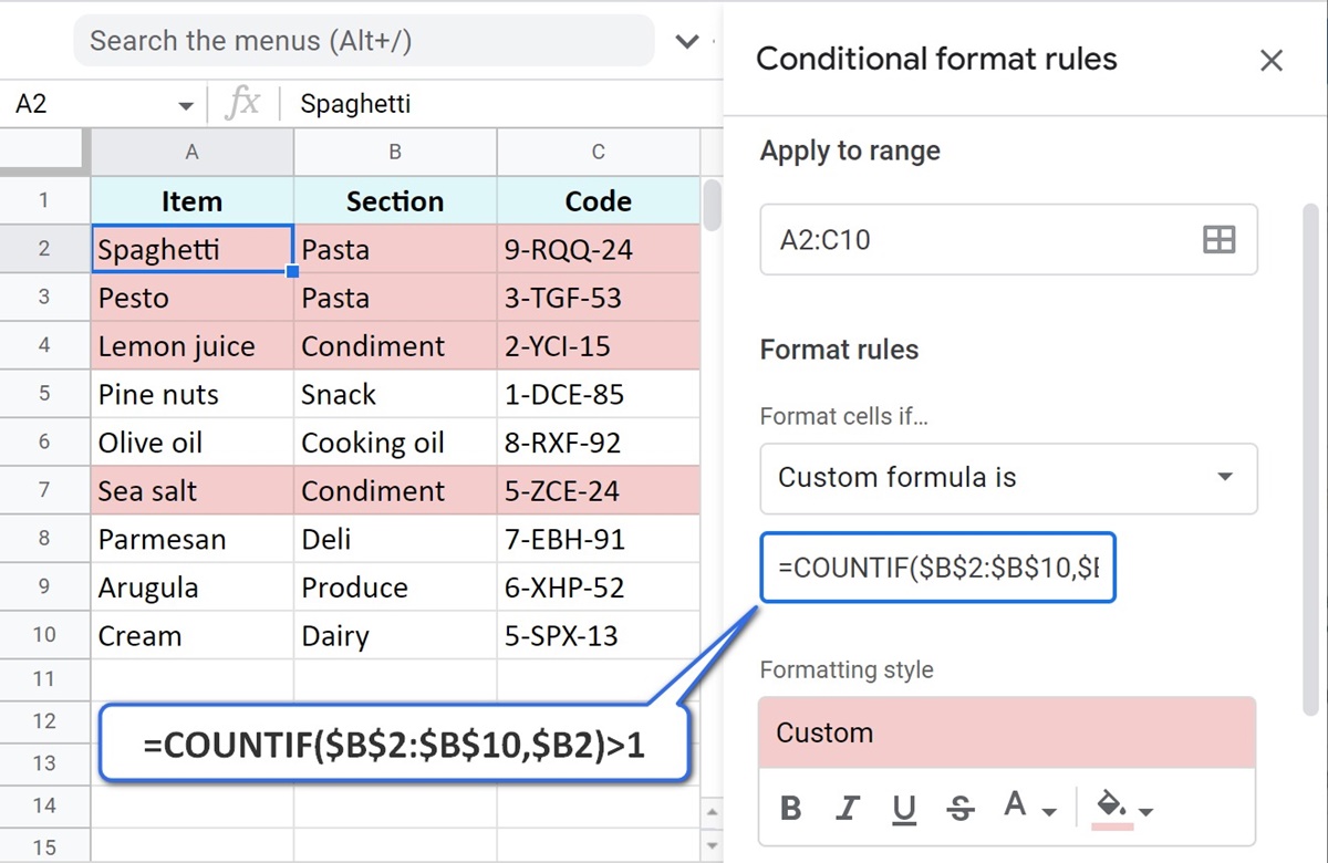
Method 1: Using Conditional Formatting
Conditional formatting is a feature in Google Sheets that allows you to apply formatting rules based on specific criteria. To highlight duplicates using conditional formatting, follow these steps:
- Select the range of cells you want to check for duplicates.
- Go to Format > Conditional formatting in the menu.
- In the conditional formatting rules panel, select Duplicate from the dropdown menu.
- Choose a formatting style to apply to the duplicate values.
- Click Done to apply the conditional formatting rules.
Now, any duplicate values in the selected range will be highlighted according to the formatting style you chose.
Method 2: Using the COUNTIF Function
The COUNTIF function allows you to count the number of occurrences of a specific value within a range. By utilizing the COUNTIF function, you can identify duplicates in your data. Here’s how:
- In an empty column next to your data, enter the formula
=COUNTIF(A:A, A1)(assuming your data is in column A and starts from row 1). - Drag the fill handle of the formula down to apply it to the entire range of data.
- Any cell with a value higher than 1 indicates a duplicate.
- Apply conditional formatting to highlight the cells with a count higher than 1.
With the help of the COUNTIF function, you can easily spot and highlight duplicate values in Google Sheets.
Method 3: Using the UNIQUE Function
The UNIQUE function in Google Sheets returns unique values from a range. By using the UNIQUE function, you can compare the original data with the unique values to identify duplicates. Follow these steps:
- In an empty column next to your data, enter the formula
=UNIQUE(A:A)(assuming your data is in column A). - In another empty column, enter the formula
=COUNTIF($A$2:$A$100, A1)(adjust the range as per your data). - Apply conditional formatting to highlight any count greater than 1.
This method allows you to find duplicates by comparing the unique values to the original data and highlight them accordingly.
Method 4: Using the FILTER Function
The FILTER function in Google Sheets allows you to filter and extract specific data from a range based on certain criteria. To identify duplicates using the FILTER function, follow these steps:
- In an empty column next to your data, enter the formula
=FILTER(A:A, COUNTIF(A:A, A:A) > 1). - This formula filters and displays the duplicate values in the data range.
- Apply conditional formatting to highlight the cells with the duplicate values.
The FILTER function offers a flexible way to identify and highlight duplicate values in Google Sheets.
Method 5: Using the Vlookup Function
The VLOOKUP function in Google Sheets allows you to search for a value in a range and retrieve data from a different column. By utilizing the VLOOKUP function, you can check if a value appears more than once and highlight the duplicates. Here’s how:
- In an empty column next to your data, enter the formula
=IF(VLOOKUP(A1, A:A, 2, FALSE) = "", "", "Duplicate")(assuming your data is in column A). - Drag the fill handle of the formula down to apply it to the entire range of data.
- The word “Duplicate” will appear in the cells with duplicate values.
- Apply conditional formatting to highlight the cells with the word “Duplicate”.
The VLOOKUP function can be a handy tool for finding and highlighting duplicate values in Google Sheets.
With these five methods, you can easily identify and highlight duplicate values in Google Sheets. Choose the method that best suits your needs to effectively manage your data and ensure data accuracy.
Method 1: Using Conditional Formatting
Conditional formatting is a powerful feature in Google Sheets that allows you to apply formatting rules based on specific criteria. With conditional formatting, you can easily highlight duplicate values in your data. Here’s how you can use this method:
- Select the range of cells that you want to check for duplicates. This can be a single column or multiple columns.
- Go to the Format menu and click on Conditional formatting. The conditional formatting rules panel will appear on the right side of the screen.
- In the conditional formatting rules panel, choose Duplicate from the dropdown menu. This option will automatically highlight any duplicate values in the selected range.
- Choose a formatting style to apply to the duplicate values. You can select a predefined formatting style or create a custom style to fit your preferences.
- Click Done to apply the conditional formatting rules. The cells containing duplicate values will now be visually distinguished according to the formatting style you selected.
Conditional formatting makes it easy to quickly identify and visually highlight duplicate values in your Google Sheets. The duplicates will be clearly marked, making it easier for you to analyze the data and take any necessary actions.
Conditional formatting can be especially useful when working with large datasets or complex spreadsheets. It allows you to visually identify duplicate values without manually searching through each cell. By applying the appropriate formatting, you can make the duplicates stand out and focus your attention on them.
Furthermore, conditional formatting is dynamic and will update automatically if any changes are made to the data. This means that if new duplicate values are added or existing duplicates are removed, the formatting will adjust accordingly. You don’t have to manually update the formatting rules every time the data changes.
Overall, using conditional formatting is an efficient and user-friendly method to highlight duplicate values in Google Sheets. It saves time and effort, allowing you to focus on analyzing the data and making informed decisions based on the information at hand.
Remember to regularly check for duplicate values in your spreadsheets to ensure data accuracy and prevent any potential errors. Utilize conditional formatting as a valuable tool in your data management process to keep your data organized and easy to interpret.
Method 2: Using the COUNTIF Function
The COUNTIF function in Google Sheets allows you to count the number of occurrences of a specific value within a range. By leveraging the power of the COUNTIF function, you can easily identify duplicate values in your data. Here’s how you can use this method:
- In an empty column next to your data, enter the formula
=COUNTIF(A:A, A1)(assuming your data is in column A and starts from row 1). - Drag the fill handle of the formula down to apply it to the entire range of data.
- Any cell with a value greater than 1 indicates a duplicate value.
- Apply conditional formatting to highlight the cells with a count greater than 1.
Using the COUNTIF function, you can easily determine how many times each value appears in your data. If a value appears more than once, it signifies a duplicate. By applying conditional formatting, you can visually highlight these duplicate values for easy identification.
It’s important to note that in the COUNTIF formula, the range is set as the entire column (e.g., A:A). This ensures that the formula covers all the cells in the column, even if the data expands in the future. Additionally, the cell reference in the formula (e.g., A1) is relative, allowing it to adjust accordingly when applied to other cells in the column.
This method is particularly useful when working with a large dataset or multiple columns of data. The COUNTIF function provides a straightforward approach to determine the presence of duplicate values without the need for complex formulas or manual searching.
By highlighting the cells with duplicate values, you can easily spot areas where data may need to be reviewed or revised. This helps you maintain data accuracy and identify any data inconsistencies or errors that may exist.
Utilizing the power of the COUNTIF function paired with conditional formatting is an efficient way to detect and highlight duplicate values in Google Sheets. It simplifies the process of identifying duplicates and allows you to focus on analyzing the data and drawing insights from it.
Remember to regularly check for duplicate values in your data to ensure data integrity. By utilizing various methods like the COUNTIF function, you can effectively manage your data and make informed decisions based on accurate information.
Method 3: Using the UNIQUE Function
The UNIQUE function in Google Sheets is a powerful tool that allows you to extract unique values from a range of data. By utilizing the UNIQUE function, you can easily identify duplicate values and highlight them for further analysis. Here’s how you can use this method:
- In an empty column next to your data, enter the formula
=UNIQUE(A:A)(assuming your data is in column A). This formula will generate a list of unique values from the column. - In another empty column, enter the formula
=COUNTIF($A$2:$A$100, A1)(adjust the range as per your data). This formula counts the number of occurrences of each value in the original column. - Apply conditional formatting to highlight any count greater than 1. This will visually distinguish the duplicate values in the original data.
By using the UNIQUE function, you can extract the unique values from your data, making it easier to spot any duplicate entries. The COUNTIF formula then compares each value in the unique list to the original data, counting how many times each unique value appears. Any value with a count greater than 1 indicates a duplicate entry.
Applying conditional formatting to the duplicate values allows you to visually highlight them, making it easier to identify and focus on areas of concern within your data.
The UNIQUE function is particularly useful when working with larger datasets or multiple columns. It simplifies the process of finding duplicate values by generating a clear list of unique entries that can be easily compared to the original data.
Additionally, the UNIQUE function is dynamic and automatically adjusts if new duplicate values are added or existing duplicates are removed. This means that the list of unique values and the corresponding conditional formatting will update accordingly, ensuring that you always have an accurate representation of the duplicates in your data.
By using the UNIQUE function in combination with conditional formatting, you can quickly identify and highlight duplicate values in your Google Sheets. This method streamlines the process of data analysis and helps ensure data accuracy for better decision-making.
Regularly checking for duplicates in your data is crucial to maintain data integrity and prevent any issues that may arise from duplicate entries. Utilize the power of the UNIQUE function along with conditional formatting to keep your data organized and identify any data inconsistencies with ease.
Method 4: Using the FILTER Function
The FILTER function in Google Sheets is a versatile tool that allows you to extract specific data from a range based on specified criteria. By utilizing the FILTER function, you can easily identify and highlight duplicate values in your data. Here’s how you can use this method:
- In an empty column next to your data, enter the formula
=FILTER(A:A, COUNTIF(A:A, A:A) > 1). This formula filters the data based on the condition that the count of each value in column A is greater than 1. - The filtered column will display the duplicate values from the original data.
- Apply conditional formatting to highlight the cells with the duplicate values in the filtered column.
By using the FILTER function and applying the appropriate criteria, you can extract the duplicate values from the original data, making them easily identifiable and distinguishable.
The FILTER function allows you to handle larger datasets or multiple columns efficiently. It filters the data based on the condition specified in the formula, providing a streamlined view of the duplicate values.
With the aid of conditional formatting, the duplicated cells in the filtered column can be highlighted, enabling you to visually spot and focus on areas where data may need to be reviewed or revised.
An advantage of using the FILTER function is that it dynamically updates as changes are made to the original data. This means that if new duplicate values are added or existing ones are removed, the filtered column will adjust automatically, reflecting any updates in the duplicate values within your data.
This approach gives you a clear, organized view of the duplicate values in a separate column, allowing for easy analysis and identification of patterns or discrepancies in the data.
By utilizing the power of the FILTER function along with conditional formatting, you can efficiently identify and highlight duplicate values in Google Sheets. This method simplifies the process of data analysis and facilitates data accuracy, ensuring that duplicated entries are readily noticeable and can be addressed promptly.
Don’t forget to regularly check for duplicate values in your data to maintain data integrity and prevent any potential errors. Utilize the FILTER function and conditional formatting as essential tools to streamline your data management process and facilitate informed decision-making.
Method 5: Using the VLOOKUP Function
The VLOOKUP function in Google Sheets is a powerful tool that allows you to search for a value in a range and retrieve corresponding data from another column. By utilizing the VLOOKUP function, you can easily identify duplicate values and highlight them for further analysis. Here’s how you can use this method:
- In an empty column next to your data, enter the formula
=IF(VLOOKUP(A1, A:A, 2, FALSE) = "", "", "Duplicate")(assuming your data is in column A). This formula searches for each value in column A and returns the corresponding value from the second column if a match is found. - Drag the fill handle of the formula down to apply it to the entire range of data.
- The word “Duplicate” will appear in the cells with duplicate values in the new column.
- Apply conditional formatting to highlight the cells with the word “Duplicate”.
The VLOOKUP function allows you to compare each value in the column with the rest of the data and determine if it appears more than once. If a match is found, indicating a duplicate value, the word “Duplicate” will be displayed in the respective cell in the new column.
By applying conditional formatting to the cells with the word “Duplicate”, you can visually highlight the duplicate values for easy identification and analysis.
The VLOOKUP function is particularly useful when you want to compare values in one column to another and retrieve related information. In this case, it helps you identify duplicate values and flag them for further attention.
This method provides a clear indication of the duplicate values in a separate column, allowing you to easily focus on areas where data may need to be reviewed or revised.
It’s worth noting that the VLOOKUP function is dynamic and will update automatically if changes are made to the data. This means that if new duplicate values are added or existing duplicates are removed, the word “Duplicate” will appear in the corresponding cells, and the conditional formatting will adjust accordingly.
By leveraging the power of the VLOOKUP function along with conditional formatting, you can efficiently identify and highlight duplicate values in Google Sheets. This method simplifies the process of data analysis and helps to ensure data accuracy.
Regularly checking for duplicates in your data is crucial to maintaining data integrity. By utilizing various methods, including the VLOOKUP function and conditional formatting, you can effectively manage your data and make informed decisions based on accurate information.
Finding Duplicate Values in Google Sheets
Duplicate values in a dataset can lead to errors and inconsistencies in your data analysis. Google Sheets provides several methods to help you easily find duplicate values, allowing you to identify and address any data redundancies. Here are five methods you can use to find duplicate values in Google Sheets:
Method 1: Using the COUNTIF Function
The COUNTIF function is a versatile tool that allows you to count the number of occurrences of a specific value within a range. By utilizing the COUNTIF function, you can easily identify duplicate values. Here’s how:
- Select the range of cells that you want to check for duplicates.
- Use the formula
=COUNTIF(A:A, A1)(assuming your data is in column A and starts from row 1) in an empty column next to your data to count the occurrences. - Any cell with a value higher than 1 indicates a duplicate value.
Method 2: Using the Pivot Table Feature
The Pivot Table feature in Google Sheets allows you to summarize and analyze large datasets. It can also help you find duplicate values. Here’s how:
- Select your data range.
- Go to the Data menu, click on Pivot Table, and choose a location for your Pivot Table.
- Add the desired column to the Rows section of the Pivot Table editor.
- In the Values section, add the same column using the Count function.
- Any count value greater than 1 indicates a duplicate value.
Method 3: Using the Filter Function
The Filter function in Google Sheets allows you to extract specific data from a range based on certain criteria. It can also be used to find duplicate values. Here’s how:
- Select the range of cells that you want to check for duplicates.
- Use the formula
=FILTER(A:A, COUNTIF(A:A, A:A) > 1)in an empty column next to your data to return the duplicate values.
Method 4: Using the UNIQUE Function
The UNIQUE function in Google Sheets returns unique values from a range. By utilizing the UNIQUE function, you can compare the original data with the unique values to identify duplicates. Here’s how:
- In an empty column next to your data, use the formula
=UNIQUE(A:A)(assuming your data is in column A). - Use the formula
=COUNTIF($A$2:$A$100, A1)(adjust the range as per your data) in another empty column to count the occurrences of each unique value.
Method 5: Using a Custom Formula
If none of the above methods suit your needs, you can create a custom formula using logical operators and functions like IF, AND, and COUNTIF to find duplicate values. Here’s an example:
- In an empty column next to your data, use the formula
=IF(COUNTIF(A:A, A1)>1, "Duplicate", "")(assuming your data is in column A).
These methods provide different approaches to help you find duplicate values in your Google Sheets. Choose the method that suits your needs and analyze your data more effectively by eliminating any duplicates and ensuring data accuracy.
Method 1: Using the COUNTIF Function
The COUNTIF function in Google Sheets is a powerful tool that allows you to count the number of occurrences of a specific value within a given range. By utilizing the COUNTIF function, you can easily identify duplicate values in your data. Here’s how you can use this method:
- Select the range of cells that you want to check for duplicates. This range can be a single column, multiple columns, or an entire dataset.
- In an empty column next to your data, enter the formula
=COUNTIF(A:A, A1)(assuming your data is in column A and starts from row 1). - Drag the fill handle of the formula down to apply it to the entire range of data.
- Any cell with a value greater than 1 indicates a duplicate value.
The COUNTIF function compares each cell in the specified range to the value in the corresponding cell. If a match is found, it increments the count by 1. By checking for values greater than 1, you can easily identify cells with duplicate values.
This method is particularly useful when working with datasets of any size. It allows you to quickly identify duplicate values without the need for complex formulas or manual searching.
Once you have identified the cells with duplicate values, you can take further action to handle them. This may involve removing the duplicates, flagging them for review, or performing additional analysis to understand the impact of the duplicates on your data.
By utilizing the power of the COUNTIF function, you can efficiently identify and manage duplicate values in your Google Sheets. This method saves time and effort, allowing you to focus on analyzing and interpreting your data accurately.
Remember to regularly check for duplicate values in your data to maintain data integrity and ensure accurate results. Utilize the COUNTIF function as a valuable tool in your data management process to eliminate duplicates and improve the quality of your data analysis.
Method 2: Using the Pivot Table Feature
The Pivot Table feature in Google Sheets is a powerful tool that allows you to summarize and analyze large datasets. It can also be used to efficiently find duplicate values within your data. Here’s how you can use this method:
- Select the range of cells that you want to check for duplicates. This can be a single column or multiple columns.
- Go to the Data menu, click on Pivot Table, and choose a location for your Pivot Table.
- In the Pivot Table editor, add the desired column to the Rows section.
- In the Values section, add the same column using the Count function. This will count the number of occurrences of each value in the selected column.
- Any count value greater than 1 indicates a duplicate value.
The Pivot Table feature allows you to summarize and organize your data, making it easier to identify duplicate values. By adding the desired column to the Rows section, you create a categorized view of your data.
The Count function in the Values section counts how many times each value appears in the selected column. Values with a count greater than 1 indicate duplicates.
By using the Pivot Table feature, you can quickly visualize the duplicate values in your dataset. This method is particularly useful when working with large datasets or when you want to gain a summarized view of your data.
Once you have identified the duplicate values, you can take appropriate actions such as removing the duplicates, investigating the reasons for duplication, or analyzing the impact of duplicates on your data analysis.
The Pivot Table feature offers the advantage of flexibility, allowing you to customize the view of your data by adding more columns, applying filters, or performing calculations. This makes it a versatile tool for data analysis and duplicate value detection.
By utilizing the Pivot Table feature in Google Sheets, you can efficiently identify and manage duplicate values in your dataset. This method simplifies the process of duplicate value detection and enables you to focus on interpreting and drawing insights from your data.
Remember to regularly check for duplicate values in your data to ensure data integrity and accurate analysis. Utilize the Pivot Table feature as a valuable tool in your data management process to identify and handle duplicate values effectively.
Method 3: Using the Filter Function
The Filter function in Google Sheets is a powerful tool that allows you to extract specific data from a range based on certain criteria. It can also be used to find duplicate values efficiently. Here’s how you can use this method:
- Select the range of cells that you want to check for duplicates. This can be a single column or multiple columns.
- In an empty column next to your data, enter the formula
=FILTER(A:A, COUNTIF(A:A, A:A) > 1)(assuming your data is in column A). This formula filters the data based on the condition that the count of each value in column A is greater than 1. - The filtered column will display the duplicate values from the original data.
The Filter function allows you to extract specific data from a range based on the criteria you set. In this case, the criteria is the condition that the count of each value in the column is greater than 1, indicating a duplicate.
By using the Filter function, the duplicate values are isolated in a separate column, making them easily identifiable. This method is particularly useful when working with large datasets or when you need to perform further analysis exclusively on the duplicate values.
Once you have identified the duplicate values, you can take appropriate actions such as removing the duplicates, investigating the source of duplication, or analyzing the impact of duplicates on your data analysis.
An advantage of using the Filter function is that it is dynamic and responsive to any changes in the data. If new duplicate values are added or existing duplicates are removed, the filtered column will automatically update to reflect these changes, ensuring accurate results.
This method provides a clear and concise view of the duplicate values in a separate column, allowing for easy analysis and identification of patterns or discrepancies in the data.
By utilizing the power of the Filter function, you can efficiently find and manage duplicate values in your Google Sheets. This method simplifies the process of duplicate value detection, enabling you to focus on analyzing and interpreting your data accurately.
Remember to regularly check for duplicate values in your data to ensure data integrity and accurate analysis. Utilize the Filter function as a valuable tool in your data management process to identify and handle duplicate values effectively.
Method 4: Using the UNIQUE Function
The UNIQUE function in Google Sheets is a powerful tool that allows you to extract unique values from a range of data. However, it can also be used to detect duplicate values efficiently. Here’s how you can use this method:
- In an empty column next to your data, enter the formula
=UNIQUE(A:A)(assuming your data is in column A). - In another empty column, enter the formula
=COUNTIF($A$2:$A$100, A1)(adjust the range as per your data). This formula counts the number of occurrences of each unique value in the original data. - Apply conditional formatting to highlight any count greater than 1. This will visually distinguish the duplicate values in the original data.
By using the UNIQUE function, you can extract the unique values from your data and compare them to the original data to identify duplicates. The COUNTIF formula counts the occurrences of each unique value, and any count greater than 1 indicates a duplicate value.
Applying conditional formatting to the cells with a count greater than 1 visually highlights the duplicate values in the original data, making them easily identifiable.
The UNIQUE function is particularly useful when working with datasets of any size. It simplifies the process of finding duplicates by generating a list of unique entries that can be easily compared to the original data.
With the help of conditional formatting, the duplicate values in the original data are easily distinguishable, allowing you to focus on areas where data may need to be reviewed or revised.
An advantage of using the UNIQUE function is that it is dynamic. If new duplicate values are added or existing duplicates are removed, the list of unique values and the conditional formatting will update automatically, ensuring that you always have an accurate representation of the duplicates in your data.
By utilizing the power of the UNIQUE function along with conditional formatting, you can efficiently identify and highlight duplicate values in Google Sheets. This method simplifies the process of duplicate value detection and allows you to focus on analyzing and interpreting your data accurately.
Remember to regularly check for duplicate values in your data to maintain data integrity and ensure accurate analysis. Utilize the UNIQUE function as a valuable tool in your data management process to identify and handle duplicate values effectively.
Method 5: Using a Custom Formula
If the previous methods don’t suit your needs, you can create a custom formula using logical operators and functions like IF, AND, and COUNTIF to find duplicate values. This approach gives you more flexibility and control over the criteria for identifying duplicates. Here’s an example of how you can use a custom formula to find duplicate values:
- In an empty column next to your data, enter the formula
=IF(COUNTIF(A:A, A1)>1, "Duplicate", "")(assuming your data is in column A).
The custom formula uses the COUNTIF function to check if a value appears more than once in the column. If the count is greater than 1, the formula returns the word “Duplicate”; otherwise, it returns an empty string.
By using a custom formula, you have the freedom to define your own conditions for identifying duplicates. You can add additional logic or criteria to further refine the identification process, depending on your specific requirements.
Once you have applied the custom formula, the cells with duplicate values will be labeled as “Duplicate” in the respective cells of the new column. This labeling can help you easily identify and take action on the duplicate values within your dataset.
After identifying the duplicate values, you can decide on the appropriate action to take. You might choose to remove the duplicates, investigate the cause of duplication, or perform additional analysis to understand the impact of duplicates on your data analysis.
A benefit of using a custom formula is that it provides a tailored solution to finding duplicates based on your unique criteria. You can adapt the formula as needed to suit different scenarios and datasets.
By utilizing a custom formula to find duplicate values in Google Sheets, you gain more control over the identification process and can focus on analyzing and managing your data effectively.
Remember to regularly check for duplicate values in your data to ensure data integrity and accurate analysis. Utilize custom formulas as a valuable tool in your data management process to identify and handle duplicate values efficiently.
Removing Duplicate Values in Google Sheets
Duplicate values can clutter your data and create inconsistencies that can affect your analysis. Google Sheets provides several methods to help you remove duplicate values and ensure data accuracy. Here are five methods you can use to remove duplicate values in Google Sheets:
Method 1: Using the Remove Duplicates Feature
Google Sheets has a built-in feature that allows you to easily remove duplicate values. Here’s how you can use this method:
- Select the range of cells that you want to remove duplicate values from.
- Go to the Data menu, click on Remove duplicates, and choose the desired columns to remove duplicates from.
- Click Remove duplicates to remove the duplicate values from the selected range.
This method automatically identifies and removes duplicate values from the selected range, leaving only unique values. It is a quick and convenient way to ensure data accuracy and eliminate duplicates.
Method 2: Using a Custom Formula
If you prefer a more customized approach, you can use a custom formula to remove duplicate values. Here’s an example of how to do this:
- In an empty column next to your data, enter the formula
=UNIQUE(A:A)(assuming your data is in column A). - Select the column with the unique values, copy it, and then paste it over the original data column using the Paste special > Paste values only option.
This method creates a column with only unique values and replaces the original data column with these unique values. It effectively removes duplicate values while preserving the rest of your data.
Method 3: Using the Query Function
The Query function in Google Sheets allows you to extract specific data from a range based on certain criteria. Here’s how you can use this method to remove duplicate values:
- In an empty column next to your data, enter the formula
=QUERY(A:A, "select A where A is not null group by A")(assuming your data is in column A). - Copy the result column, paste it as values only, and then paste it back over the original data column.
This method uses the Query function to group the data by each unique value in column A and returns only the unique values. Copying and pasting as values over the original data column eliminates duplicates while preserving the integrity of your data.
Method 4: Using the UNIQUE Function
The UNIQUE function in Google Sheets allows you to extract unique values from a range. Here’s how you can remove duplicates using this method:
- In an empty column next to your data, enter the formula
=UNIQUE(A:A)(assuming your data is in column A). - Select and copy the column with unique values.
- Paste the copied column over the original data column using the Paste special > Paste values only option.
This method uses the UNIQUE function to create a column with only unique values. Pasting the unique values over the original data column effectively removes duplicates and maintains the overall structure of your data.
Method 5: Using the Filter Function
The Filter function in Google Sheets allows you to extract specific data from a range based on certain criteria. Here’s how you can use this method to remove duplicates:
- In an empty column next to your data, enter the formula
=FILTER(A:A, COUNTIF(A:A, A:A) = 1)(assuming your data is in column A). - Select and copy the filtered column.
- Paste the copied column over the original data column using the Paste special > Paste values only option.
This method uses the Filter function to create a column with only unique values. Pasting the filtered column over the original data column removes the duplicates, leaving only unique values behind.
By utilizing these methods, you can easily remove duplicate values in your Google Sheets and ensure data accuracy. Choose the method that suits your needs and maintain a clean and reliable dataset for efficient data analysis.
Method 1: Using the Remove Duplicates Feature
Duplicate values can complicate data analysis and impact the accuracy of your results. Google Sheets provides a convenient built-in feature that allows you to quickly remove duplicate values. Here’s how you can use this method:
- Select the range of cells that you want to remove duplicate values from. This can be a single column or multiple columns.
- Go to the Data menu and click on Remove duplicates.
- In the Remove duplicates dialog box, select the columns you want to consider for finding duplicates. By default, all columns are selected.
- Click the Remove duplicates button to delete duplicate values from the selected range.
The Remove duplicates feature scans the selected range and removes any duplicate values, keeping only the unique values. This ensures that your data remains clean and free of redundant entries.
This method is ideal for quickly eliminating duplicate values, especially when working with large datasets. It saves time and effort by automating the process of identifying and removing duplicates.
When duplicates are removed, the original order of the data is preserved, and the remaining unique values are repositioned accordingly. This allows you to maintain the integrity and structure of your dataset.
It is important to exercise caution when using this feature, as it permanently deletes duplicate values without the ability to undo the action. Therefore, it’s recommended to create a backup or copy of your data before using this method, especially when dealing with critical or irrecoverable information.
By utilizing the Remove duplicates feature in Google Sheets, you can efficiently clean your data, ensuring accurate analysis and reliable results.
Regularly checking for and removing duplicate values is essential to maintain the integrity of your data. By utilizing the built-in Remove duplicates feature, you can easily manage and clean your data to enhance the accuracy and effectiveness of your data analysis efforts.
Method 2: Using a Custom Formula
If you prefer a more tailored approach to remove duplicate values, you can use a custom formula in Google Sheets. This method gives you greater flexibility and control over the criteria for identifying duplicates. Here’s how you can use this method:
- In an empty column next to your data, enter the formula
=UNIQUE(A:A)(assuming your data is in column A). - Select and copy the column with the unique values.
- Paste the copied column over the original data column using the Paste special > Paste values only option.
This custom formula approach uses the UNIQUE function to generate a column with only the unique values from the original data column. Copying and pasting the unique values over the original data effectively removes the duplicate values.
By using a custom formula, you have the ability to tailor the removal of duplicates based on your specific needs. You can apply additional criteria or logic to further refine the removal process.
Using this method helps to maintain the structure and integrity of your data while eliminating any duplications. It allows you to have full control over the removal process, ensuring that only unique values remain.
It’s important to note that this method permanently removes duplicate values from your data. Therefore, it’s recommended to create a backup or copy of your data before applying the custom formula, especially when dealing with critical or irrecoverable information.
By employing a custom formula to remove duplicate values in Google Sheets, you can ensure data accuracy and optimize your data analysis. This method allows you to tailor the removal process according to your specific criteria, streamlining your data management efforts.
Regularly checking for and removing duplicate values is crucial to maintain the integrity of your data. By leveraging custom formulas, you can effectively identify and eliminate duplicates, resulting in cleaner data and more accurate analysis.
Method 3: Using the Query Function
The Query function in Google Sheets provides a powerful way to extract specific data from a range based on certain criteria. You can also utilize the Query function to remove duplicate values efficiently. Here’s how you can use this method:
- In an empty column next to your data, enter the formula
=QUERY(A:A, "select A where A is not null group by A")(assuming your data is in column A). - Copy the resulting column of unique values.
- Paste the copied column as values over the original data column, using the Paste special > Paste values only option to replace the duplicate values.
The Query function retrieves unique values from the selected data column. With the group by A clause, the function groups identical values together, resulting in a list of unique values.
Copying and pasting the resulting column of unique values as values over the original data column replaces the duplicate values with unique values, effectively removing duplicates.
The Query function is flexible and allows you to customize parameters such as applying additional conditions, sorting, or summarizing data. This enables you to fine-tune the removal of duplicates according to your specific requirements.
It’s important to note that when using the Query function, the resulting values are dynamic, meaning that if new duplicate values are added or existing duplicates are removed, the unique values will update accordingly.
Remember to create a backup or copy of your data before applying the Query function, especially when dealing with critical or irrecoverable information. This ensures that you have a safeguard in case you need to revert back to the original data.
By using the Query function to remove duplicate values in Google Sheets, you can streamline your data management process and ensure data accuracy. The flexible nature of the Query function allows you to tailor the removal process according to your specific criteria.
Regularly checking for and removing duplicate values is essential to keep your data clean and accurate. Utilize the versatile Query function to efficiently identify and remove duplicates, enabling you to maintain the integrity of your data and conduct more reliable analyses.
Method 4: Using the UNIQUE Function
The UNIQUE function in Google Sheets is a powerful tool that allows you to extract unique values from a range of data. Besides finding unique values, you can also utilize the UNIQUE function to remove duplicate values efficiently. Here’s how you can use this method:
- In an empty column next to your data, enter the formula
=UNIQUE(A:A)(assuming your data is in column A). - Select and copy the column with the unique values.
- Paste the copied column over the original data column using the Paste special > Paste values only option.
By applying the UNIQUE function, you generate a column with only the unique values from the original data column. Copying and pasting the unique values over the original data column effectively removes the duplicate values.
The UNIQUE function is particularly useful when you need to work with large datasets or multiple columns. It streamlines the process of removing duplicates by extracting the unique values automatically.
The advantage of using the UNIQUE function is that it allows you to customize your data management process. You can easily apply filters, further calculations, or other operations on the unique values as needed.
It’s important to note that this method permanently removes duplicate values from your data. Therefore, it’s recommended to create a backup or copy of your data before applying the UNIQUE function, especially when dealing with critical or irrecoverable information.
By utilizing the UNIQUE function in Google Sheets, you can efficiently remove duplicate values and ensure data accuracy. This method simplifies the process of removing duplicates, allowing you to focus on analyzing and interpreting your data effectively.
Regularly checking for and removing duplicate values is crucial in maintaining accurate and reliable data. Incorporate the UNIQUE function into your data management process to eliminate duplicates and optimize the quality of your data analysis.
Method 5: Using the Filter Function
The Filter function in Google Sheets is a versatile tool that allows you to extract specific data from a range based on certain criteria. It can also be used effectively to remove duplicate values. Here’s how you can use this method:
- In an empty column next to your data, enter the formula
=FILTER(A:A, COUNTIF(A:A, A:A) = 1)(assuming your data is in column A). - Select and copy the filtered column.
- Paste the copied column as values over the original data column using the Paste special > Paste values only option.
Using the Filter function, you can create a column that only contains the unique values from the original data. The formula COUNTIF(A:A, A:A) = 1 filters the data to only include values that appear once, effectively removing the duplicates.
Copying and pasting the filtered column as values over the original data column replaces the duplicate values with the unique values, removing any redundancy while preserving the integrity of your data.
The Filter function provides flexibility, as you can customize the criteria to suit your needs. For example, you can add additional conditions or combine it with other functions to further refine the removal process.
It’s important to note that this method permanently removes duplicate values from your data. It’s recommended to create a backup or copy of your data before using the Filter function, especially when dealing with critical or irrecoverable information.
By utilizing the power of the Filter function in Google Sheets, you can efficiently remove duplicate values and ensure data accuracy. This method allows you to focus on analyzing and interpreting your data without the distraction of redundant entries.
Regularly checking for and removing duplicate values is essential for maintaining clean and reliable data. Utilize the Filter function as a valuable tool in your data management process to make your data analysis more precise and impactful.