
Highlighting Cells Based on Text
Conditional formatting is a powerful feature in Google Sheets that allows you to automatically highlight cells based on their text values. This can be incredibly useful for visually organizing and analyzing your data. Here’s how you can use conditional formatting to highlight cells based on text:
1. Select the range of cells you want to apply the formatting to. You can do this by clicking and dragging the mouse over the desired cells.
2. Go to the “Format” menu and choose “Conditional formatting.”
3. In the conditional formatting sidebar that appears on the right, select “Text contains” from the dropdown menu.
4. Enter the specific text that you want to highlight. For example, if you want to highlight cells that contain the word “Completed,” type “Completed” in the text box.
5. Choose the formatting style that you want to apply to the highlighted cells. You can change the font color, background color, or add a custom format.
6. Click the “Done” button to apply the conditional formatting to the selected range of cells.
Once you have applied the conditional formatting, any cell that contains the specified text will be highlighted according to your chosen formatting style. This can make it easier to identify and analyze specific data points in your sheet.
For example, if you are tracking the progress of tasks in a project management sheet, you can use conditional formatting to highlight cells that contain keywords like “In progress,” “Pending,” or “Completed.” This will give you a visual representation of the current status of each task.
Conditional formatting based on text can also be used to identify patterns or anomalies in your data. For instance, you can highlight cells that contain certain keywords or phrases to quickly identify common themes or outliers.
With the ability to highlight cells based on text, Google Sheets’ conditional formatting features provide a powerful tool for data visualization and analysis. By using these formatting options effectively, you can make your spreadsheets more visually appealing and easy to interpret.
Highlighting Cells Based on Numbers
Conditional formatting in Google Sheets not only allows you to highlight cells based on text, but it also offers the ability to highlight cells based on numerical values. This feature can be particularly useful when working with data sets that require visual analysis. Here’s how you can use conditional formatting to highlight cells based on numbers:
1. Select the range of cells you want to apply the formatting to. You can do this by clicking and dragging the mouse over the desired cells.
2. Go to the “Format” menu and choose “Conditional formatting.”
3. In the conditional formatting sidebar, select “Greater than,” “Less than,” or any other comparison option based on your specific requirements.
4. Enter the value you want to use for comparison. For example, if you want to highlight cells that have values greater than 100, enter “100” in the input box.
5. Choose the formatting style that you want to apply to the highlighted cells. This can include changing the font color, background color, or applying a custom format.
6. Click the “Done” button to apply the conditional formatting to the selected range of cells.
Once you have applied the conditional formatting, any cell that meets the specified numerical condition will be highlighted according to your chosen formatting style. This can help you quickly identify trends, outliers, or specific data points within your sheet.
For example, if you have a sales sheet and you want to identify all sales transactions that exceed a certain threshold, you can use conditional formatting to highlight cells with values greater than a specified amount. This will allow you to easily spot the high-value sales transactions.
Conditional formatting based on numbers can also be used for other purposes, such as highlighting cells that fall within a specific range or identifying cells that have negative values.
By leveraging conditional formatting in Google Sheets, you can effectively visually analyze numerical data and gain valuable insights. The ability to highlight cells based on numbers provides a dynamic way to identify patterns and draw attention to important data points within your spreadsheet.
Highlighting Cells Based on Dates
Conditional formatting in Google Sheets allows you to highlight cells based on dates, helping you to organize and analyze time-based data more effectively. Whether you’re managing project deadlines, tracking sales figures, or monitoring events, conditional formatting can be a valuable tool. Here’s how you can highlight cells based on dates:
1. Select the range of cells you want to apply the formatting to. This can be done by clicking and dragging the mouse over the desired cells.
2. Go to the “Format” menu and choose “Conditional formatting.”
3. In the conditional formatting sidebar, select “Date is” from the dropdown menu.
4. Choose the specific conditions you want to apply based on dates. For example, you can select “Today,” “Yesterday,” “This week,” or specify a custom date range.
5. Choose the formatting style you want to apply to the highlighted cells, such as changing font color, background color, or adding a custom format.
6. Click the “Done” button to apply the conditional formatting to the selected range of cells.
Once you have applied the conditional formatting, cells that meet the specified date conditions will be highlighted according to your chosen formatting style. This allows you to easily identify dates that fall within certain parameters.
For instance, if you have a project management sheet and want to track upcoming deadlines, you can use conditional formatting to highlight cells with dates approaching the current day. This way, you’ll be able to quickly identify tasks that require immediate attention.
Conditional formatting based on dates can also be helpful when analyzing trends or patterns. For example, you can highlight all cells that have dates falling within a certain month or quarter to identify periods of high activity or low activity.
By utilizing conditional formatting in Google Sheets, you can effectively manage and analyze time-based data. The ability to highlight cells based on dates provides a visual representation of your data, helping you make informed decisions and prioritize tasks.
Highlighting Cells Based on Formulas
Conditional formatting in Google Sheets not only allows you to highlight cells based on their values, text, or dates, but it also provides the flexibility to highlight cells based on formulas. This feature enables you to create custom rules that dictate when certain cells should be highlighted, depending on the evaluation of formulas. Here’s how you can use conditional formatting to highlight cells based on formulas:
1. Select the range of cells you want to apply the formatting to. You can do this by clicking and dragging the mouse over the desired cells.
2. Go to the “Format” menu and choose “Conditional formatting.”
3. In the conditional formatting sidebar, select “Custom formula is” from the dropdown menu.
4. Enter the formula that you want to use as the conditions for highlighting cells. For example, if you want to highlight cells where the value is greater than the average of a specific range, you can use a formula like “=A1 > AVERAGE(A2:A10)”.
5. Choose the formatting style that you want to apply to the highlighted cells, such as changing the font color, background color, or adding a custom format.
6. Click the “Done” button to apply the conditional formatting to the selected range of cells.
Once you have applied the conditional formatting, cells that meet the specified formula condition will be highlighted according to your chosen formatting style. This allows you to visually identify cells that satisfy complex calculations or logical conditions.
Conditional formatting based on formulas can be incredibly powerful in data analysis. You can use formulas to compare values, calculate percentages, evaluate text conditions, and much more. By highlighting cells based on these formulas, you can easily identify outliers, trends, or specific data points that meet your specific criteria.
For example, you can use conditional formatting with formulas to highlight cells in a sales sheet where the revenue exceeds a certain percentage of the target. This will help you identify successful sales transactions and potentially focus on areas that need improvement.
By leveraging the customizable nature of conditional formatting and using formulas, you can gain deep insights into your data and highlight cells based on complex calculations. This feature in Google Sheets provides a powerful tool for analyzing and visualizing data in a dynamic and intuitive way.
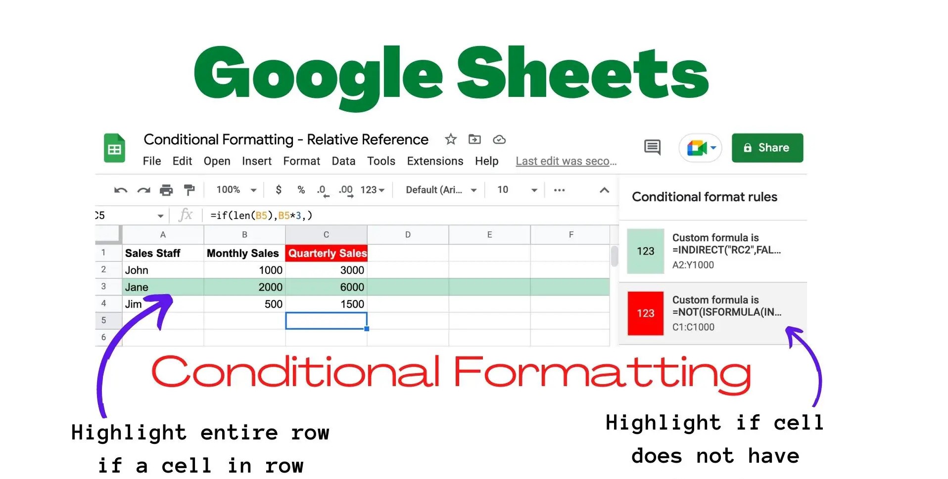
Highlighting an Entire Row Based on a Cell Value
Conditional formatting in Google Sheets not only allows you to highlight individual cells based on certain criteria, but it also provides the capability to highlight entire rows based on the value of a specific cell. This can be particularly useful to visually emphasize specific data or identify patterns within a spreadsheet. Here’s how you can highlight an entire row based on a cell value:
1. Select the range of cells you want to apply the formatting to. This range should include the entire table or dataset where you want to highlight rows.
2. Go to the “Format” menu and choose “Conditional formatting.”
3. In the conditional formatting sidebar, select “Custom formula is” from the dropdown menu.
4. Enter the formula to check the value of the cell in the first column of the selected row. For example, if you want to highlight rows where the value in column A is “Completed,” you can use a formula similar to “=A1 = “Completed”.” Note that the cell reference (A1) should correspond to the first cell of the selected range.
5. Choose the formatting style you want to apply to the entire row. This can include changing the font color, background color, or adding a custom format.
6. Click the “Done” button to apply the conditional formatting to the selected range of cells.
Once you have applied the conditional formatting, any row that meets the specified criteria will be highlighted according to your chosen formatting style. This allows you to easily identify and focus on rows that contain specific values in a particular column.
For instance, if you have a spreadsheet for inventory management, you can highlight entire rows where the quantity of a certain product is below a desired threshold. This makes it easier to identify low-stock items and take appropriate actions.
Highlighting entire rows based on a cell value can also be useful when working with survey responses or data entries. You can highlight rows where a specific answer is selected or where certain conditions are met, making it easier to analyze and extract information from the dataset.
By using conditional formatting to highlight entire rows based on a cell value, you can quickly visually identify important information, patterns, or specific data points within your spreadsheet. This can help streamline your data analysis and improve the overall efficiency of your workflow.
Creating Your Own Conditional Formatting Rules
In addition to the predefined options in Google Sheets’ conditional formatting, you have the flexibility to create your own custom conditional formatting rules. This allows you to tailor the formatting to your specific needs and preferences. Here’s how you can create your own conditional formatting rules:
1. Select the range of cells you want to apply the formatting to. You can do this by clicking and dragging the mouse over the desired cells.
2. Go to the “Format” menu and choose “Conditional formatting.”
3. In the conditional formatting sidebar, select the “Custom formula is” option from the dropdown menu.
4. Enter the formula that defines the condition for formatting. This can be any valid formula using cell references and various operators. For instance, you can use formulas like “=A1 > B1” to compare the values of two cells, or “=LEN(A1) > 5” to check if the length of a cell’s content exceeds a certain limit.
5. Choose the formatting style that you want to apply to the cells that meet your custom formula condition. This can include changing the font color, background color, or applying a custom format.
6. Click the “Done” button to apply the conditional formatting to the selected range of cells.
Once you have created your custom conditional formatting rule, the cells that meet the specified condition will be formatted accordingly. This gives you the ability to apply complex logic and formatting options to highlight specific data points in your sheet.
For example, let’s say you have a spreadsheet tracking employee performance, and you want to highlight cells where the performance rating is above a certain threshold. You can create a custom rule using a formula like “=C1 > 8” to highlight cells with a rating greater than 8.
Creating your own conditional formatting rules gives you the flexibility to adapt the formatting to your specific requirements. You can use various formulas to create rules based on different conditions, comparisons, or calculations. This empowers you to truly customize your spreadsheet and make your data analysis more effective.
By leveraging custom conditional formatting rules, you can visually highlight important information, identify trends or outliers, and gain valuable insights from your data with ease.
Copying Conditional Formatting Rules
Copying conditional formatting rules in Google Sheets can save you time and effort when you want to apply the same formatting to multiple ranges or sheets within your spreadsheet. This feature allows you to easily replicate your conditional formatting settings without having to manually recreate them each time. Here’s how you can copy conditional formatting rules:
1. Select the range or sheet that contains the conditional formatting rule you want to copy.
2. Go to the “Format” menu and choose “Conditional formatting.”
3. In the conditional formatting sidebar, click on the “Cell range” dropdown menu to view the options.
4. Select the range or sheet where you want to apply the same conditional formatting rule. You can choose a specific range or select an entire sheet.
5. Click the “Done” button to close the conditional formatting sidebar.
Once you have copied the conditional formatting rule, it will be applied to the selected range or sheet. This will replicate the same formatting settings, including the formatting style and the formula or condition used.
This feature is particularly useful when you have created a complex conditional formatting rule or if you want to maintain consistency in the formatting across different parts of your spreadsheet.
For example, if you have applied conditional formatting to highlight overdue tasks in one sheet, you can easily copy the formatting rule to other sheets in your spreadsheet. This helps ensure a uniform formatting style and allows you to quickly identify overdue tasks throughout the entire document.
Copying conditional formatting rules also comes in handy when you need to apply the same formatting to multiple ranges within a sheet. Instead of manually recreating the rule for each range, you can copy the rule and paste it to the desired ranges, saving you valuable time and effort.
By using the copy and paste feature for conditional formatting rules in Google Sheets, you can streamline your formatting process and maintain consistency across your spreadsheet. This allows you to easily apply complex formatting rules to multiple ranges or sheets, enhancing the visual organization and analysis of your data.
Clearing Conditional Formatting Rules
In Google Sheets, you have the option to clear conditional formatting rules when you no longer need them or want to start fresh with formatting. Clearing these rules allows you to remove the applied formatting and revert the cells back to their default formatting. Here’s how you can clear conditional formatting rules:
1. Select the range of cells or sheet where you want to clear the conditional formatting rules.
2. Go to the “Format” menu and choose “Conditional formatting.”
3. In the conditional formatting sidebar, click on the “Cell range” dropdown menu to view the options.
4. Select the range or sheet where you want to clear the conditional formatting rules. You can choose a specific range or select an entire sheet.
5. Click the “Clear rules” button located at the top right corner of the conditional formatting sidebar.
6. In the dialog box that appears, select “Clear formatting rules” to remove all conditional formatting rules from the selected range or sheet.
Once you have cleared the conditional formatting rules, the applied formatting will be removed, and the cells will revert to their default formatting style. This allows you to start fresh or apply new conditional formatting rules as needed.
Clearing conditional formatting rules is useful when you no longer require the formatting, want to simplify your spreadsheet, or need to apply a new set of formatting rules that best meet your current requirements.
For example, if you have applied conditional formatting to highlight specific data points in a sheet, but later decide to change the criteria for highlighting, you can clear the existing rules and create new ones based on the updated requirements.
Clearing conditional formatting rules also comes in handy when you want to remove all formatting from a sheet and return it to its default appearance. This can be helpful when sharing your spreadsheet with others or when you want to present the information without any applied formatting.
By being able to clear conditional formatting rules in Google Sheets, you have the flexibility to modify and adjust your formatting as needed, while maintaining control over the visual organization and presentation of your data.