
What is a drop-down list in Excel?
A drop-down list in Excel is a feature that allows you to create a selection menu within a cell or a group of cells. It provides a set of predefined options that users can choose from, rather than typing in data manually. When you click on the cell, a drop-down arrow appears, and upon clicking it, a list of choices is displayed. The user can then select an option by simply clicking on it.
Drop-down lists are commonly used in Excel for various purposes, such as data validation, form creation, and data entry. They offer a convenient and efficient way to restrict input to a predefined set of values, ensuring consistency and accuracy in data entry. Whether you are creating a simple personal budget or a complex inventory management system, drop-down lists can greatly enhance your Excel spreadsheets’ functionality.
Drop-down lists can be customized to fit your specific needs. You can control the selection options and their order, define input messages to guide users, and even set up error alerts for invalid entries. With a drop-down list, you can streamline data entry, minimize errors, and make your worksheets more user-friendly.
Excel provides a range of options for creating drop-down lists, giving you the flexibility to adapt them to your specific requirements. Whether you’re a beginner or an experienced user, mastering the creation and management of drop-down lists in Excel will undoubtedly boost your productivity and improve the quality of your data.
Why use a drop-down list in Excel?
Using a drop-down list in Excel offers numerous advantages and benefits that can greatly enhance your spreadsheet’s functionality and efficiency. Here are some compelling reasons to utilize drop-down lists:
1. Data Validation: Drop-down lists provide a practical way to enforce data validation rules. By limiting the choices to predefined options, you can ensure that the entered data is accurate and consistent. This helps to prevent errors, typos, and invalid entries.
2. Efficiency and Accuracy: With a drop-down list, users can quickly select the desired value from a predefined set of options, eliminating the need for manual typing. This increases the speed and accuracy of data entry, reducing the chances of mistakes and saving valuable time.
3. Consistency: By restricting the choices to a specific list, drop-down lists promote data consistency throughout your spreadsheet. This uniformity ensures that all entries follow the same format and meet the required criteria. It helps to maintain data integrity and facilitates data analysis and reporting.
4. User-Friendly Interface: Drop-down lists provide a user-friendly interface, making it easier for users to enter data correctly. The visual aspect of the drop-down menu, along with clear choices, simplifies the input process and reduces the learning curve for new users.
5. Error Prevention and Alerts: Excel allows you to set up error alerts when invalid entries are made in a drop-down list. You can configure custom error messages to notify users of the data entry mistake and guide them towards making the correct selection. This proactive approach helps to prevent errors before they become larger issues.
6. Customizability and Flexibility: Drop-down lists in Excel are highly customizable. You can easily modify the list of options, change the order of items, or even link the list to a range of cells for dynamic updates. This flexibility allows you to adapt the drop-down list to your specific needs and requirements.
By leveraging the power of drop-down lists in Excel, you can enhance data entry, improve accuracy, and create a more efficient workflow. Whether you’re managing a project, tracking inventory, or organizing customer data, drop-down lists are a valuable tool in your Excel arsenal.
How to create a drop-down list in Excel
Creating a drop-down list in Excel is a straightforward process that can be accomplished in a few simple steps. Follow the steps below to create your own drop-down list:
Step 1: Select the cell(s) where you want to create the drop-down list. Choose the cell or a range of cells where you want the drop-down list to appear. This is the cell that users will click on to access the list of options.
Step 2: Go to the Data tab on the Excel ribbon. Navigate to the Data tab located at the top of the Excel window.
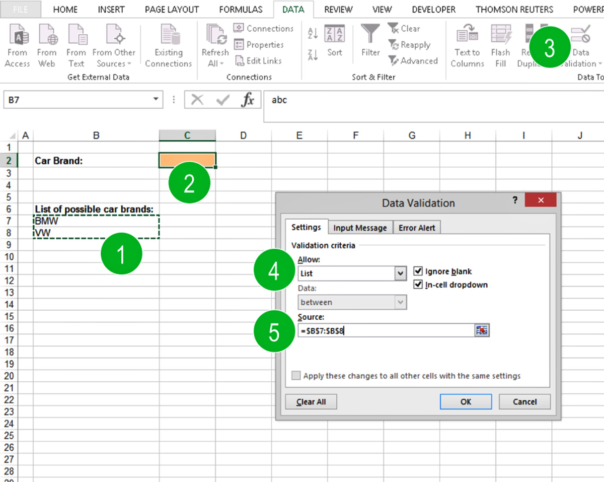
Step 3: Click on the Data Validation button. In the Data Tools group, click on the “Data Validation” button. This will open the Data Validation dialog box.
Step 4: Choose the Validation tab in the Data Validation dialog box. In the Data Validation dialog box, make sure the “Settings” tab is selected. This is where you will define the rules for your drop-down list.
Step 5: Select “List” in the Allow drop-down menu. In the Allow drop-down menu, choose the option “List.” This tells Excel that you want to create a drop-down list.
Step 6: Enter the list of items in the “Source” field. In the Source field, enter the items you want to include in the drop-down list. You can type the items directly into the field, separate them by commas, or refer to a range of cells that contains the options.
Step 7: Customize the input message and error alert (optional). If desired, you can customize the input message and error alert that appear when users interact with the drop-down list. The input message can serve as a helpful hint or instruction, while the error alert can provide guidance if an invalid entry is made.
Step 8: Click OK to create the drop-down list. Once you are satisfied with the settings and the list of options, click OK to create the drop-down list. The selected cell or cells will now display a drop-down arrow, indicating that a list of choices is available.
That’s it! You have successfully created a drop-down list in Excel. You can now test it by clicking on the cell and selecting one of the options from the drop-down menu.
Note that you can modify or remove the drop-down list at any time by accessing the Data Validation dialog box and adjusting the settings accordingly. With a drop-down list in place, you can streamline data entry, improve accuracy, and make your Excel worksheets more user-friendly.
Step 1: Select the cell(s) where you want to create the drop-down list
The first step in creating a drop-down list in Excel is to select the cell or range of cells where you want the drop-down list to appear. This is the cell that users will click on to access the list of options.
Here’s how you can select the cell(s) for your drop-down list:
1. Click on the cell: Start by clicking on the cell where you want the drop-down list to be located. If you want to create a drop-down list in multiple adjacent cells, click and drag to select the entire range.
2. Select multiple non-adjacent cells (optional): If you want to create a drop-down list in multiple non-adjacent cells, hold down the Ctrl key on your keyboard while clicking on the desired cells. This will allow you to select multiple cells at once.
3. Extend the selection: If you have already selected a single cell and want to extend the selection to adjacent cells, hold down the Shift key on your keyboard and use the arrow keys to expand the selection in the desired direction.
4. Select a range of cells: If you want to create a drop-down list in a range of cells that are not adjacent, select the first cell in the range, hold down the Shift key, and click on the last cell of the range.
5. Collapse the selection: If you have selected a large range of cells and want to collapse the selection back to a single cell, press the Esc key on your keyboard.
By following these steps, you can easily select the cell(s) where you want to create your drop-down list in Excel. Remember that the selected cell(s) will display a drop-down arrow after you have successfully created the drop-down list, indicating that a list of choices is available for selection.
Now that you have completed Step 1, you can proceed to the next steps to create and customize your drop-down list in Excel.
Step 2: Go to the Data tab on the Excel ribbon
After selecting the cell(s) where you want to create the drop-down list, the next step is to navigate to the Data tab on the Excel ribbon. This tab contains the necessary tools and options for data-related tasks, including creating a drop-down list.
Here’s how you can access the Data tab:
1. Open Excel and locate the ribbon: Launch Excel and open the workbook in which you want to create the drop-down list. The ribbon is the horizontal strip at the top of the Excel window, consisting of various tabs.
2. Find and click on the Data tab: Look for the Data tab on the ribbon. The tabs are organized based on different categories such as File, Home, Insert, etc. Click on the Data tab, which is typically located between the Formulas and Review tabs.
3. Review the options on the Data tab: Once you are on the Data tab, take a moment to familiarize yourself with the available options. These options are specifically designed to work with data-related tasks, including data validation, sorting, filtering, and more.
By accessing the Data tab on the Excel ribbon, you are now ready to proceed to the next step in creating your drop-down list. The Data tab provides you with the necessary tools and functions to define the rules and settings for your drop-down list, making it a crucial step in the process.
Continue to the next section for Step 3, where you will learn how to click on the Data Validation button to further customize your drop-down list.
Step 3: Click on the Data Validation button
Once you have navigated to the Data tab on the Excel ribbon, the next step in creating a drop-down list is to click on the Data Validation button. This button allows you to define validation rules and set up the drop-down list.
Here’s how you can access the Data Validation button:
1. Locate the Data Tools group: On the Data tab, look for the Data Tools group. This group usually contains options related to data validation, sorting, and filtering.
2. Find the Data Validation button: Within the Data Tools group, you will find the Data Validation button. It is represented by an icon that resembles a green board with a white checkmark and an arrow facing downwards. Click on this button to open the Data Validation dialog box.
3. Familiarize yourself with the options: Once you click on the Data Validation button, the Data Validation dialog box will appear. This dialog box allows you to set up various validation rules, including creating the drop-down list. Take a moment to review the available tabs and options within the dialog box.
By clicking on the Data Validation button, you have accessed the Data Validation dialog box, which is where you will define the rules and settings for your drop-down list. This step is essential for creating and customizing the behavior of the drop-down list, such as the list source, input restriction, and error messages.
Next, proceed to Step 4 to learn how to choose the Validation tab within the Data Validation dialog box.
Step 4: Choose the Validation tab in the Data Validation dialog box
After clicking on the Data Validation button, the next step in creating a drop-down list is to choose the Validation tab within the Data Validation dialog box. This tab contains options for setting up validation rules and specifying the type of data allowed in the selected cell(s).
Here’s how you can select the Validation tab:
1. Open the Data Validation dialog box: When you click on the Data Validation button in the Data Tools group on the Data tab, the Data Validation dialog box will appear on your screen.
2. Locate the Validation tab: Within the Data Validation dialog box, you will find multiple tabs. Choose the tab labeled “Validation” to access the options specifically related to data validation.
3. Review the options on the Validation tab: Once you are on the Validation tab, you will see different settings that allow you to define the desired behavior for the drop-down list. These settings include the validation criteria, input message, and error alert.
By selecting the Validation tab in the Data Validation dialog box, you are now ready to proceed with the next steps in configuring your drop-down list. This step is crucial as it assists in specifying the validation rules and customizing the behavior of the drop-down list based on your requirements.
Continue to Step 5 to learn how to choose the “List” option in the Allow drop-down menu, which is the next stage in creating your drop-down list in Excel.
Step 5: Select “List” in the Allow drop-down menu
After accessing the Validation tab within the Data Validation dialog box, the next step in creating a drop-down list is to select the “List” option in the Allow drop-down menu. This option allows you to specify that you want to create a drop-down list in the selected cell(s) that contains a predefined set of choices.
Follow these steps to select the “List” option:
1. Open the Data Validation dialog box: Click on the Data Validation button in the Data Tools group on the Data tab to open the Data Validation dialog box.
2. Navigate to the Validation tab: Within the Data Validation dialog box, make sure the Validation tab is selected. This is where you define the validation rules.
3. Choose “List” from the Allow drop-down menu: In the Allow drop-down menu, click on the option labeled “List.” By selecting this option, you inform Excel that you want to create a drop-down list.
By selecting the “List” option in the Allow drop-down menu, you have specified that you want to create a drop-down list in the selected cell(s). This signifies that the cell will display a drop-down arrow, indicating the presence of a list of choices that users can select from.
Continue to Step 6 to learn how to enter the list of items in the “Source” field, which is necessary to populate your drop-down list with the desired choices.
Step 6: Enter the list of items in the “Source” field
After selecting the “List” option in the Allow drop-down menu, the next step in creating a drop-down list is to enter the list of items in the “Source” field. This field specifies the options that will populate the drop-down list for users to choose from.
Follow these steps to enter the list of items in the “Source” field:
1. Open the Data Validation dialog box: Click on the Data Validation button in the Data Tools group on the Data tab to open the Data Validation dialog box.
2. Go to the Validation tab: Within the Data Validation dialog box, make sure the Validation tab is selected.
3. Enter the list of items: In the Source field, enter the list of items you want to include in the drop-down list. You can type the items directly into the field, separating them by commas (e.g., Item1, Item2, Item3) or other appropriate delimiters.
Note: Alternatively, you can specify a range of cells that contain the items you want to include in the drop-down list. To do this, click on the “Select range” button (represented by a small grid icon) next to the Source field, and then select the desired range of cells.
After entering the list of items in the “Source” field, the drop-down list will be populated with these options. When users click on the cell with the drop-down arrow, they will see the list of choices you have entered.
Now that you have completed Step 6, proceed to Step 7 to learn how to customize the input message and error alert options in the Data Validation dialog box. These options can provide additional guidance and validation for users interacting with the drop-down list.
Step 7: Customize the input message and error alert (optional)
After entering the list of items in the “Source” field, the next step in creating a drop-down list is to customize the input message and error alert. These options, while optional, can provide valuable guidance and validation for users interacting with the drop-down list.
Follow these steps to customize the input message and error alert:
1. Open the Data Validation dialog box: Click on the Data Validation button in the Data Tools group on the Data tab to open the Data Validation dialog box.
2. Navigate to the Validation tab: Within the Data Validation dialog box, make sure the Validation tab is selected.
3. Input message (optional): If you want to provide an input message to guide users when they interact with the drop-down list, check the “Show input message when cell is selected” checkbox. Then, enter a title and a message in the respective fields. The input message will be displayed as a pop-up when the user clicks on the cell with the drop-down arrow.
4. Error alert (optional): To set up an error alert in case an invalid entry is made in the drop-down list, check the “Show error alert after invalid data is entered” checkbox. Select the desired style of error alert from the drop-down menu, such as “Stop,” “Warning,” or “Information.” Then, enter a title and an error message in the respective fields. The error alert will be displayed if the user tries to enter data that is not part of the drop-down list.
Note: By default, Excel prevents users from entering invalid data when a drop-down list is enforced. However, customizing the input message and error alert provides additional guidance and feedback.
After customizing the input message and error alert, users will receive helpful messages and alerts when they interact with the drop-down list. This can effectively guide them towards making correct and valid entries.
Proceed to Step 8 to complete the process of creating a drop-down list in Excel, where you will click OK to finalize the settings and apply the drop-down list to the selected cell(s).
Step 8: Click OK to create the drop-down list
After customizing the input message and error alert (if desired), the final step in creating a drop-down list in Excel is to click OK. This action will confirm your settings and apply the drop-down list to the selected cell(s).
Follow these steps to complete the process:
1. Open the Data Validation dialog box: Click on the Data Validation button in the Data Tools group on the Data tab to open the Data Validation dialog box.
2. Review the settings: Double-check the settings you have configured, including the list source, input message, and error alert. Ensure that everything is set up to your satisfaction.
3. Click OK: Once you are ready to create the drop-down list, click the OK button in the Data Validation dialog box. This action will finalize the settings and apply the drop-down list to the selected cell(s).
After clicking OK, you will notice that the selected cell(s) now display a drop-down arrow. This arrow indicates the presence of a drop-down list, and upon clicking it, users will see the list of options you have defined.
Congratulations! You have successfully created a drop-down list in Excel. Users can now select from the predefined choices you have specified, promoting data accuracy and streamlining data entry tasks.
Remember that you can modify or remove the drop-down list at any time by accessing the Data Validation dialog box and adjusting the settings accordingly. This gives you the flexibility to update or customize your drop-down list as needed.
Now that you have completed all the necessary steps, you can enjoy the benefits of using a drop-down list in Excel to enhance your data entry and improve the efficiency of your spreadsheets.
How to edit or remove a drop-down list in Excel
Once you have created a drop-down list in Excel, you may find the need to edit or remove it in the future. Excel provides easy-to-use tools that allow you to make changes to the drop-down list according to your requirements. Here’s how you can edit or remove a drop-down list:
Editing the items in the drop-down list:
To edit the items in the drop-down list, follow these steps:
1. Select the cell(s) containing the drop-down list: Click on the cell(s) where the drop-down list is located to select it. If the drop-down list spans multiple cells, select the entire range.
2. Go to the Data tab: Navigate to the Data tab on the Excel ribbon. This is where you’ll find the necessary tools for editing the drop-down list.
3. Click on the Data Validation button: In the Data Tools group on the Data tab, click on the “Data Validation” button. This will open the Data Validation dialog box.
4. Modify the list items: Within the Data Validation dialog box, you can make changes to the list of items in the “Source” field. Edit the items as needed, adding or removing options as required.
5. Click OK: Once you have finished editing the items in the drop-down list, click the OK button in the Data Validation dialog box to save the changes.
Your drop-down list will now reflect the modifications you made to the items. Users will see the updated options when they interact with the drop-down list.
Removing the drop-down list:
If you wish to remove the drop-down list completely, follow these steps:
1. Select the cell(s) containing the drop-down list: Click on the cell(s) where the drop-down list is located to select it. If the drop-down list spans multiple cells, select the entire range.
2. Go to the Data tab: Navigate to the Data tab on the Excel ribbon.
3. Click on the Data Validation button: In the Data Tools group on the Data tab, click on the “Data Validation” button. This will open the Data Validation dialog box.
4. Clear the validation: Within the Data Validation dialog box, click on the “Clear All” button. This will remove the data validation rule, including the drop-down list, from the selected cell(s).
5. Click OK: Once you have cleared the validation, click the OK button in the Data Validation dialog box to finalize the removal of the drop-down list.
The drop-down list will no longer be present in the selected cell(s). Users will be able to enter any value they desire into those cells.
By understanding how to edit or remove a drop-down list in Excel, you have the ability to modify and manage your data validation effectively. Whether you need to update the options in the drop-down list or completely remove it, Excel provides the necessary tools to accomplish these tasks with ease.
Editing the items in the drop-down list
Excel allows you to easily edit the items in a drop-down list to accommodate changes or updates. Whether you need to add new options, remove existing ones, or modify the order of items, editing the drop-down list can be done in a few simple steps. Here’s how you can edit the items in a drop-down list:
1. Select the cell(s) containing the drop-down list: Start by selecting the cell or range of cells where the drop-down list is located. Click on the cell(s) to highlight them. If the list spans multiple cells, select the entire range.
2. Go to the Data tab on the Excel ribbon: Navigate to the Data tab, which is located at the top of the Excel window. This is where you’ll find the necessary options for editing the drop-down list.
3. Click on the Data Validation button: In the Data Tools group on the Data tab, click on the “Data Validation” button. This will open the Data Validation dialog box, where you can make changes to the drop-down list.
4. Modify the list items: Within the Data Validation dialog box, you’ll see the “Source” field. This is where the items for the drop-down list are defined. Edit the items in the “Source” field to add, remove, or modify the existing options. Separate each item with a comma if there are multiple items.
5. Click OK to save the changes: Once you have finished editing the items in the drop-down list, click the OK button in the Data Validation dialog box to save and apply the changes.
By following these steps, you can easily update the items in the drop-down list to reflect any changes or updates that may be required. Whether you need to add new items, remove outdated options, or adjust the arrangement of the list, Excel provides a user-friendly interface to make these modifications.
Remember to ensure that your modified drop-down list is still valid and meets the necessary criteria for your data entry or validation purposes. Regularly reviewing and updating the drop-down list ensures accuracy and relevance in your Excel spreadsheets.
Removing the drop-down listIf you no longer need a drop-down list in your Excel spreadsheet, you can easily remove it. Removing the drop-down list allows users to freely input any value into the selected cell(s) without any restriction or predefined choices. Here’s how you can remove a drop-down list:
1. Select the cell(s) containing the drop-down list: Begin by selecting the cell or range of cells where the drop-down list is located. Click on the cell(s) to highlight them. If the list spans multiple cells, select the entire range.
2. Go to the Data tab on the Excel ribbon: Navigate to the Data tab, located at the top of the Excel window. This tab provides access to the necessary options for removing the drop-down list.
3. Click on the Data Validation button: In the Data Tools group on the Data tab, click on the “Data Validation” button. This will open the Data Validation dialog box, where you can manage the data validation settings.
4. Clear the validation: Within the Data Validation dialog box, click on the “Clear All” button. This removes the data validation rule, including the drop-down list, from the selected cell(s). The content of the previously selected cell(s) will no longer be restricted to the options in the drop-down list.
5. Click OK to finalize the removal: Once you have cleared the validation and removed the drop-down list, click the OK button in the Data Validation dialog box to finalize the changes.
After following these steps, the drop-down list will be completely removed from the selected cell(s). Users will no longer see a list of predefined options when interacting with those cells, and they will be able to freely input any value.
Removing a drop-down list can be useful when the specific data validation or input restriction is no longer needed or when you want to provide more flexibility for data entry. Keep in mind that you can always recreate the drop-down list if necessary and update it with new options or modified criteria.
Tips and tricks for working with drop-down lists in Excel
Working with drop-down lists in Excel can greatly enhance data entry and improve the usability of your spreadsheets. Here are some tips and tricks to help you make the most out of drop-down lists:
1. Adding new items to the drop-down list: To add new items to an existing drop-down list, simply edit the “Source” field in the Data Validation dialog box. Separate each item with a comma or specify a range of cells for the new options.
2. Changing the order of items in the drop-down list: If you want to change the order of items in the drop-down list, edit the “Source” field in the desired order. The drop-down list will reflect the updated order of options.
3. Using a range of cells as the source for the drop-down list: Instead of manually entering the list of items in the “Source” field, you can select a range of cells with the desired items. This allows for easier management and dynamic updates if the range contents are changed.
4. Customizing the appearance of the drop-down arrow: You can modify the appearance of the drop-down arrow by changing the font or selecting a different symbol for the cell(s) containing the drop-down list. This can help differentiate the drop-down cells from other regular cells.
5. Ensuring data integrity with error alerts: Utilize the error alert feature to provide users with informative messages when an invalid entry is made. Consider using a “Stop” style error alert to prevent incorrect data from being entered in the first place.
6. Protecting the drop-down list: If you want to protect the drop-down list from accidental modification, consider protecting the worksheet or locking the cells containing the drop-down list. This helps maintain the integrity of the list while permitting users to interact with it.
7. Using data validation formulas: Explore advanced data validation options by utilizing formulas in the Data Validation dialog box. This allows for more complex validations based on specific criteria in your Excel formulas.
8. Creating dependent drop-down lists: Use data validation with formulas and named ranges to create dependent or cascading drop-down lists. This allows you to filter the choices in one drop-down list based on the selection made in another list.
9. Testing the drop-down list: Always test the drop-down list after creating or modifying it to ensure that it functions as intended. Verify the options, sequencing, and error alerts to guarantee a seamless user experience.
10. Documenting the drop-down list: Consider adding a comment or cell note to provide instructions or information about the drop-down list. This helps users understand the purpose and required input for the drop-down list.
By applying these tips and tricks, you can maximize the effectiveness of drop-down lists in Excel, promoting data accuracy, efficient data entry, and improved usability in your spreadsheets.
Adding new items to the drop-down list
Adding new items to an existing drop-down list in Excel is a straightforward process that allows you to expand and update the choices available. By adding new items, you can ensure that your drop-down list remains relevant and up to date. Here’s how you can add new items to a drop-down list:
1. Select the cell(s) containing the drop-down list: Begin by selecting the cell or range of cells where the drop-down list is located. Click on the cell(s) to highlight them. If the list spans multiple cells, select the entire range.
2. Go to the Data tab on the Excel ribbon: Navigate to the Data tab, located at the top of the Excel window. This tab provides access to the necessary options for managing drop-down lists.
3. Click on the Data Validation button: In the Data Tools group on the Data tab, click on the “Data Validation” button. This will open the Data Validation dialog box.
4. Edit the “Source” field: Within the Data Validation dialog box, locate the “Source” field. This field contains the existing list of items for the drop-down list. Append or insert new items within this field, ensuring that each item is separated by a comma or other appropriate delimiter.
5. Click OK to save the changes: Once you have added the new items to the drop-down list, click the OK button in the Data Validation dialog box to save and apply the changes.
After following these steps, the drop-down list will now include the newly added items. Users will see these additional choices when interacting with the drop-down list.
Adding new items to a drop-down list allows you to expand the available options and adapt the list to evolving needs. This flexibility ensures that your drop-down list remains comprehensive and provides users with the most relevant choices for data entry or selection.
Changing the order of items in the drop-down list
In Excel, changing the order of items in a drop-down list allows you to customize the sequence in which options appear. By rearranging the order, you can prioritize certain choices or group related items together. Here’s how you can change the order of items in a drop-down list:
1. Select the cell(s) containing the drop-down list: Start by selecting the cell or range of cells where the drop-down list is located. Click on the cell(s) to highlight them. If the list spans multiple cells, select the entire range.
2. Go to the Data tab on the Excel ribbon: Navigate to the Data tab, situated at the top of the Excel window. This tab provides access to a variety of data-related options, including data validation.
3. Click on the Data Validation button: In the Data Tools group on the Data tab, click on the “Data Validation” button. This will open the Data Validation dialog box.
4. Edit the “Source” field: Within the Data Validation dialog box, locate the “Source” field. This field contains the list of items for the drop-down list. Modify the order of items in this field to change the sequence. You can either rearrange the items manually or use cut-and-paste operations to reorder them as desired.
5. Click OK to save the changes: After rearranging the items in the drop-down list, click the OK button in the Data Validation dialog box to save and apply the changes.
Following these steps will update the drop-down list with the new order of items. Users will now see the options in the revised sequence when interacting with the drop-down list.
Changing the order of items in a drop-down list offers you the flexibility to customize and optimize the display of options. It can help make the list more intuitive or align with specific requirements, enhancing the usability and effectiveness of your Excel spreadsheets.
Using a range of cells as the source for the drop-down list
In Excel, you have the option to use a range of cells as the source for a drop-down list. By linking the drop-down list to a range of cells, you can easily update and manage the choices without modifying the data validation settings. Here’s how you can use a range of cells as the source for a drop-down list:
1. Prepare the range of cells: Prepare a range of cells that contains the items you want to include in the drop-down list. This range can be in the same worksheet or even in a different worksheet or workbook.
2. Select the cell(s) for the drop-down list: Select the cell(s) where you want the drop-down list to appear. Click on the cell(s) to highlight them. If the drop-down list spans multiple cells, select the entire range.
3. Go to the Data tab on the Excel ribbon: Navigate to the Data tab located at the top of the Excel window. This tab provides access to various data-related options.
4. Click on the Data Validation button: In the Data Tools group on the Data tab, click on the “Data Validation” button. This will open the Data Validation dialog box.
5. Enter the range in the “Source” field: Within the Data Validation dialog box, select the “List” option from the “Allow” drop-down menu. Then, in the “Source” field, enter or select the range of cells that contain the items for the drop-down list. You can either type the range in directly or click the “Select range” button to choose the range from the worksheet.
6. Click OK to save the changes: Once you have specified the range of cells as the source for the drop-down list, click the OK button in the Data Validation dialog box to save and apply the changes.
By using a range of cells as the source for the drop-down list, any changes made to the cells within that range will automatically update the options in the drop-down list. This provides a dynamic and efficient way to manage and update the choices without modifying the data validation settings each time.
Using a range of cells as the source for a drop-down list offers flexibility and convenience, especially when you have a large or frequently changing set of options. It simplifies the process of maintaining and updating the drop-down list and ensures that it always reflects the most current data in your Excel spreadsheets.
Tips for working with large drop-down lists
Working with large drop-down lists in Excel can present some challenges in terms of usability and performance. To ensure a smooth experience for users and optimal functionality, consider these helpful tips when working with large drop-down lists:
1. Use filtering options: If your drop-down list has an extensive number of items, consider enabling filtering options. This allows users to search and narrow down the options based on specific criteria, making it easier to find the desired item.
2. Arrange items alphabetically: Organize the items in alphabetical order within the drop-down list to facilitate easier and quicker navigation. This helps users easily locate and select the desired option without scrolling extensively.
3. Implement cascading drop-down lists: If your data has hierarchical relationships, consider using cascading drop-down lists. This means that the options in one drop-down list are dependent on the selection made in another, effectively narrowing down the choices and making the selection process more manageable.
4. Utilize abbreviations or codes: If your drop-down list contains long or detailed items, consider using abbreviations or codes to represent the options. This conserves space in the list and allows for quicker scanning and selection.
5. Enable autocomplete: Enable the autocomplete feature in Excel, which suggests possible matches as users start typing in the drop-down list cell. This can speed up the selection process and provide instant feedback to users.
6. Consider using a separate input sheet: For very large drop-down lists, consider using a separate sheet dedicated to listing and managing the options. This can help keep your primary worksheet uncluttered and improve performance.
7. Optimize your formulas: If you’re using formulas to generate the list items in the drop-down list, ensure that your formulas are optimized to avoid any unnecessary calculations or delays in populating the list.
8. Test performance and responsiveness: Regularly test the performance and responsiveness of your large drop-down lists, especially if they involve complex formulas or extensive data ranges. Optimize the settings or consider alternative approaches if you notice any lags or slowdowns.
9. Provide clear instructions: For large and complex drop-down lists, include clear instructions or tooltips to guide users on how to navigate, search, and select the desired options.
10. Consider alternative UI components: If the drop-down list becomes too large or unwieldy, evaluate whether alternative user interface components such as combo boxes, list boxes, or searchable dropdowns would better accommodate your data and user needs.
By following these tips, you can improve the usability and performance of large drop-down lists in Excel, ensuring an efficient and user-friendly experience for those interacting with your spreadsheets.