Create a Google Sheets Drop-Down List

What is a Google Sheets Drop-Down List?

A Google Sheets drop-down list is a feature that allows you to create a list of predefined options within a cell in your Google Sheets spreadsheet. It provides a convenient way to limit the choices users can make when entering data, ensuring consistency and accuracy.

With a drop-down list, you can specify a set of values that users can select from a menu, rather than manually typing the options. This not only saves time but also helps to avoid data entry errors. Once the drop-down list is created, users can simply click on the cell and choose an option from the provided list.

Drop-down lists are particularly useful when you have a finite number of choices or specific categories that you want to enforce in your spreadsheet. They can be applied to individual cells, entire columns, or even across multiple sheets within your Google Sheets document.

The real power of a drop-down list in Google Sheets lies in its ability to streamline data entry and ensure consistency throughout your spreadsheet. By limiting the available choices, you maintain control over the data being entered, making it easier to analyze and organize your information.

How to Create a Drop-Down List in Google Sheets

Creating a drop-down list in Google Sheets is a straightforward process that can be done in just a few steps. Here’s how to do it:

Select the cell or range of cells where you want to create the drop-down list.
Click on the “Data” tab in the menu bar and select “Data validation.”
In the data validation dialog box, choose “List from a range” or “List of items” under the “Criteria” section, depending on whether you want to create the list from a range of cells or a custom set of values.

If you choose “List from a range,” you’ll need to specify the range of cells containing the options you want to include in the drop-down list.

If you choose “List of items,” you can manually type the values you want to include in the drop-down list, separating them with commas.

Make sure the “Show dropdown list in cell” option is checked.
Click “Save” to create the drop-down list.

Once you’ve created the drop-down list, you’ll see a small arrow icon in the cell or cells you selected. Clicking on this arrow will open the drop-down menu, allowing you or other users to choose from the available options.

You can also customize the appearance and behavior of the drop-down list by modifying the data validation settings. For example, you can choose to show an error message when an invalid value is entered or even create a dependent drop-down list that changes based on the selection in another cell.

Creating drop-down lists in Google Sheets is a powerful way to streamline data entry and ensure consistency in your spreadsheets. Whether you’re managing budgets, tracking inventory, or collecting survey responses, drop-down lists can greatly improve the efficiency and accuracy of your data management process.

Creating a List from a Range of Cells

One of the ways to create a drop-down list in Google Sheets is by using a range of cells as the source of your options. This allows you to easily update the list by modifying the values in the cells. Here’s how to create a drop-down list from a range of cells:

Select the cell or range of cells where you want to create the drop-down list.
Click on the “Data” tab in the menu bar and select “Data validation.”
In the data validation dialog box, choose “List from a range” under the “Criteria” section.
In the “Range” field, enter the range of cells that contain the options you want to include in the drop-down list. For example, if your options are in cells A1 to A5, you would enter “A1:A5”.
Make sure the “Show dropdown list in cell” option is checked.
Click “Save” to create the drop-down list.

Once you’ve created the drop-down list, the values in the specified range of cells will be displayed as options in the drop-down menu. If you make any changes to the values in those cells, the drop-down list will automatically update to reflect the modified options. This makes it easy to maintain and manage your drop-down lists as your data changes over time.

Creating a drop-down list from a range of cells is particularly useful when you have a large set of options or when the list is likely to change frequently. By referencing a range of cells, you can easily update the drop-down list without having to manually modify each individual option.

Whether you’re managing data for project tracking, client lists, or product categories, creating drop-down lists from ranges of cells in Google Sheets provides a convenient way to control data entry and ensure accuracy in your spreadsheets.

Creating a List from a Custom Set of Values

In addition to creating a drop-down list in Google Sheets from a range of cells, you can also create a drop-down list using a custom set of values. This gives you the flexibility to specify the options directly without relying on the contents of a specific range of cells. Here’s how you can create a drop-down list from a custom set of values:

Select the cell or range of cells where you want to create the drop-down list.
Click on the “Data” tab in the menu bar and select “Data validation.”
In the data validation dialog box, choose “List of items” under the “Criteria” section.
In the “Items” field, enter the values you want to include in the drop-down list, separating them with commas. For example, if you’re creating a drop-down list of colors, you could enter “Red, Blue, Green, Yellow”.
Make sure the “Show dropdown list in cell” option is checked.
Click “Save” to create the drop-down list.

Once you’ve created the drop-down list, the specified values will be displayed as options in the drop-down menu. Users can select from the provided options when entering data, ensuring consistency and accuracy.

Creating a drop-down list from a custom set of values is particularly useful when you have a specific set of options that you want to enforce in your spreadsheet. It allows you to tailor the drop-down list to your specific needs without relying on external data sources.

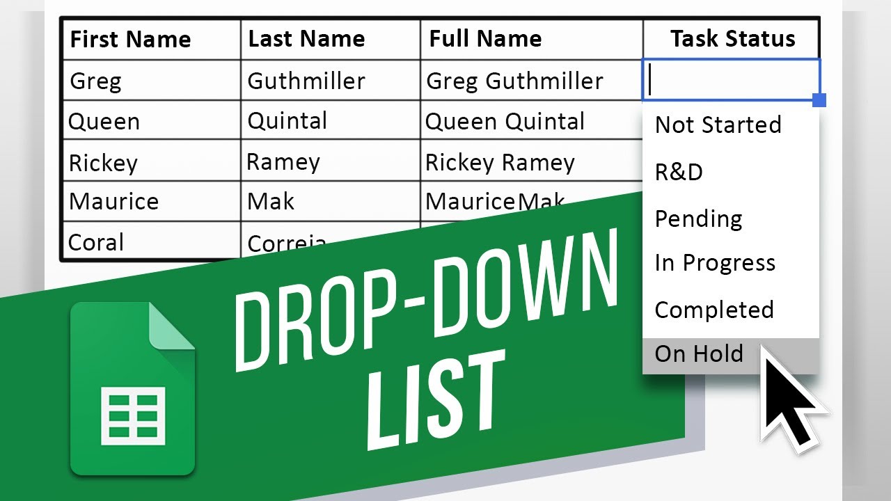
Whether you’re creating drop-down lists for product categories, project statuses, or equipment options, using a custom set of values in Google Sheets provides you with a flexible and convenient way to control data entry and ensure consistency throughout your spreadsheet.

Removing or Editing a Drop-Down List

If you want to remove or edit a drop-down list in Google Sheets, you have a couple of options depending on your needs. Here’s how you can remove or edit a drop-down list:

To remove a drop-down list:

Select the cell or range of cells that contain the drop-down list.
Click on the “Data” tab in the menu bar and select “Data validation.”
In the data validation dialog box, click on the “Remove” button.
Click “Save” to remove the drop-down list.

Once you’ve removed the drop-down list, the cell or range of cells will no longer have the drop-down functionality, and users will be able to enter any value they want manually.

To edit a drop-down list:

Select the cell or range of cells that contain the drop-down list.
Click on the “Data” tab in the menu bar and select “Data validation.”
In the data validation dialog box, make the necessary changes to the range or items in the “Criteria” section.
Click “Save” to update the drop-down list.

By editing the drop-down list, you can modify the range of cells or update the custom set of values based on your requirements.

Removing or editing a drop-down list allows you to adapt your spreadsheet to changing needs or correct any errors. Whether you need to update the options or eliminate the drop-down functionality altogether, Google Sheets provides the necessary tools to make these adjustments easily.

Using Data Validation to Limit Entry Options

Google Sheets provides a powerful feature called data validation, which allows you to go beyond drop-down lists and further control and limit the options for data entry in your spreadsheet. With data validation, you can enforce specific rules and restrictions on the values entered in a cell or range of cells. Here’s how you can use data validation to limit entry options:

Select the cell or range of cells where you want to apply data validation.
Click on the “Data” tab in the menu bar and select “Data validation.”
In the data validation dialog box, choose the validation criteria that best suit your needs.
Set the desired criteria, such as allowing only whole numbers or decimal numbers within a certain range, or requiring a specific date format.
Specify the error message to display when an invalid value is entered, providing instructions or clarification to the user.
Optional: You can also choose to show a warning message when a value that doesn’t meet the validation criteria is entered.
Click “Save” to apply the data validation.

Once data validation is applied, users will be restricted to entering values that comply with the defined criteria. If an invalid value is entered, an error message will be displayed, preventing incorrect or inconsistent data from being entered into the spreadsheet.

Data validation provides enhanced control over data entry and ensures data integrity in your spreadsheet. By limiting the available options and enforcing specific criteria, you can minimize errors, standardize data input, and ensure the accuracy and coherence of your data.

Whether you’re using data validation to restrict entry options in financial spreadsheets, project management trackers, or any other type of data collection, this feature in Google Sheets proves to be a valuable tool for maintaining clean and consistent data throughout your sheets.

Creating a Drop-Down List Dependent on Another Cell

In Google Sheets, you can create a drop-down list that is dependent on the value selected in another cell. This means that the options available in the drop-down list will change dynamically based on the value in a specific cell. This can be particularly useful when you want to create cascading or conditional drop-down lists. Here’s how you can create a drop-down list dependent on another cell:

Select the cell or range of cells where you want to create the drop-down list.
Click on the “Data” tab in the menu bar and select “Data validation.”
In the data validation dialog box, choose “List from a range” under the “Criteria” section.
In the “Range” field, enter the range of cells that contain the options for the initial drop-down list.
Make sure the “Show dropdown list in cell” option is checked.
In the “On invalid data” section, select “Reject input” or “Show warning” depending on how you want to handle invalid selections.
Check the box for “Use custom formula is” and enter the formula that will determine the range of cells for the dependent drop-down list. For example, if the initial drop-down list is in cell A1, and you want the dependent drop-down list to show options based on the selection in cell A1, then the formula could be something like “=INDIRECT(A1)”.
Click “Save” to create the drop-down list dependent on another cell.

Once you’ve set up the dependent drop-down list, the options in the drop-down menu will change automatically based on the value selected in the initial cell. This provides a dynamic and interactive way to control data entry and streamline your data collection process.

Creating a drop-down list dependent on another cell is beneficial when you have hierarchical data or when certain options are only relevant based on a previous selection. It allows you to narrow down choices for better data accuracy and to customize the options available to users based on their specific needs or context.

Whether you’re managing category selections, location choices, or any other type of conditional data entry, creating dependent drop-down lists in Google Sheets provides a powerful way to enhance data entry efficiency and ensure data consistency.

Using Color-Coding in Drop-Down Lists

Google Sheets allows you to add visual cues and improve data interpretation by using color-coding in drop-down lists. By assigning specific colors to different options in the drop-down menu, you can quickly identify and distinguish between different categories or values. Here’s how you can use color-coding in drop-down lists:

Select the cell or range of cells where you have the drop-down list.
Click on the “Format” tab in the menu bar and select “Conditional formatting.”
In the conditional formatting dialog box, choose “Single color” under the “Format cells if” section.
Choose the desired color for the option you want to format, or click “Custom formula is” for more advanced formatting options.
In the “Value or formula” field, enter the formula or value that corresponds to the option you want to format.
Click “Done” to apply the color-coding.

Once you’ve applied color-coding to the drop-down list, the options in the menu will be visually distinguishable based on the assigned colors. This makes it easier to identify specific options at a glance and provides a more intuitive way of analyzing and interpreting the data.

Color-coding can be particularly useful when working with large datasets or when there is a need to categorize and group information. For example, you can use different colors to represent different priority levels, status indicators, or product categories in your drop-down lists.

By using color-coding, you can enhance the visual aspect of your spreadsheet and make it easier for users to locate and select the desired options. It improves readability and comprehension, allowing for quicker and more accurate data analysis and decision-making.

Whether you’re managing project tasks, inventory tracking, or any other type of data organization, using color-coding in drop-down lists in Google Sheets adds an extra layer of clarity and makes your spreadsheet more visually appealing.

Tips and Tricks for Working with Drop-Down Lists in Google Sheets

Drop-down lists in Google Sheets are a powerful tool for data entry and organization. Here are some tips and tricks to help you make the most out of working with drop-down lists:

Use cell references: Instead of manually typing the options in the data validation criteria, you can refer to a range of cells that contains the options. This allows for easier editing and updating of the options without modifying each individual drop-down list.
Add a prompt message: When setting up data validation for your drop-down list, consider adding a prompt message to provide instructions or additional information to the users. This can help prevent data entry mistakes and ensure understanding.
Employ conditional formatting: Combine drop-down lists with conditional formatting to visually highlight specific cells based on the selected value. This can help bring attention to important data points or identify trends in your spreadsheet more easily.
Consider using data validation for numeric values: Data validation isn’t limited to just creating drop-down lists. You can also use it to set restrictions on numeric values such as minimum and maximum ranges, decimal or whole numbers, or even custom formulas for more complex validations.
Utilize the support of keyboard shortcuts: Google Sheets has various keyboard shortcuts that make working with drop-down lists more efficient. For example, you can press Alt + Down Arrow to open the drop-down menu, or Alt + Enter to accept the selected value and move to the next cell.
Use cell protection: To prevent accidental changes to the drop-down list or its associated data, consider protecting the cells containing the drop-down list. With cell protection, you can ensure that only authorized users can modify the list or the data within.

By implementing these tips and tricks, you can optimize your use of drop-down lists in Google Sheets, improving data entry accuracy, organization, and overall efficiency. Whether you’re managing finances, inventories, or survey responses, mastering these techniques will contribute to a smoother and more effective data management process.