
What are Worksheets and Workbooks in Excel?
Worksheets and workbooks are fundamental elements in Microsoft Excel that allow you to organize and analyze data effectively. Excel is a powerful spreadsheet program that helps you perform various calculations, create graphs and charts, and manage large sets of data.
A worksheet is a single sheet within an Excel file where you can enter, manipulate, and analyze data. It consists of a grid of cells organized into columns and rows. Each cell can contain different types of data, such as numbers, text, dates, or formulas. Worksheets provide a vast canvas for you to input and organize information in a structured manner.
A workbook, on the other hand, is a collection of multiple worksheets. It acts as a container for related data and calculations, allowing you to keep your work organized and easily accessible. Workbooks are useful when you need to separate data by categories, such as different departments, projects, or time periods.
Excel allows you to create and manage multiple worksheets within a single workbook, enabling you to perform complex data analysis and comparisons without the need for separate files. Workbooks help facilitate data organization, collaboration, and navigation, making it easier to work with different sets of data within the same file.
Worksheets and workbooks in Excel provide a versatile platform for various tasks, from simple data entry and calculations to advanced data analysis and visualization. Whether you’re a student, professional, or business owner, understanding how to effectively utilize worksheets and workbooks in Excel is essential for improving efficiency and productivity.
Creating a New Worksheet or Workbook
Creating a new worksheet or workbook in Excel is a straightforward process that allows you to start organizing and analyzing data. Whether you need to track expenses, manage inventory, or perform calculations, Excel provides the tools to create and customize your worksheets and workbooks.
To create a new worksheet, simply open Excel and click on the “Insert” tab in the menu bar. From the options displayed, click on “Worksheet.” A new blank worksheet will be inserted into your current workbook. You can also use the shortcut key “Ctrl + Shift + N” to create a new worksheet instantly.
If you need to create a new workbook, either to separate different sets of data or to start a new project, click on the “File” tab in the menu bar and select “New.” This will open the New Workbook window, where you can choose from various templates or select a blank workbook. Clicking on the “Blank Workbook” option will create a new workbook with a single blank worksheet.
Once you have created a new worksheet or workbook, you can customize it to suit your needs. You can change the name of the worksheet or workbook by double-clicking on the default name displayed at the bottom or top of the Excel window. Enter a new name and press Enter to save the changes.
Furthermore, you can format the worksheet or workbook by adjusting the column widths, selecting different fonts and colors, applying cell borders, and more. These formatting options allow you to improve the readability and visual appeal of your data.
Creating new worksheets or workbooks in Excel gives you the freedom to organize and analyze data effectively. By customizing the layout and formatting, you can create a professional-looking spreadsheet that meets your specific requirements.
Renaming a Worksheet or Workbook
In Excel, you have the flexibility to rename both worksheets and workbooks according to your preferences. Renaming allows you to give more meaningful names to your sheets or files, making it easier to identify and manage them. Whether you want to provide a descriptive name for a specific sheet or give your workbook a more recognizable title, Excel provides simple methods to rename worksheets and workbooks.
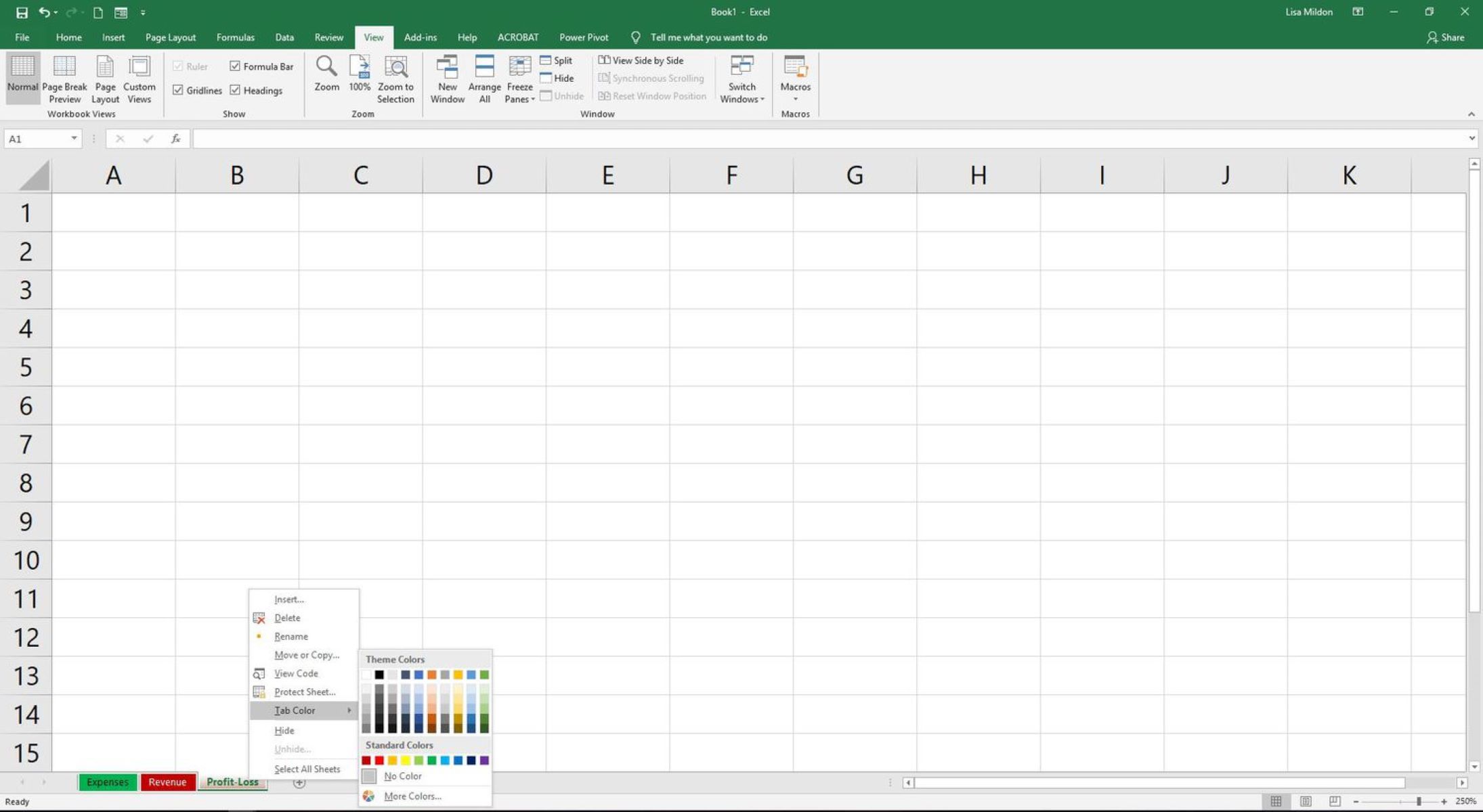
To rename a worksheet, right-click on the sheet tab at the bottom of the Excel window. From the context menu that appears, select “Rename” or simply double-click on the sheet tab. This action will activate the sheet name, allowing you to input a new name. Press Enter to save the changes, or click anywhere outside the sheet tab to exit the renaming mode.
Keep in mind that worksheet names should be unique within a workbook to distinguish each sheet. Descriptive names that reflect the content of the sheet are recommended to enhance organization and easy navigation.
Similarly, you can rename a workbook to give it a more memorable title or indicate its purpose. To change the name of a workbook, go to the “File” tab in the menu bar and select “Save As.” In the Save As window, input the desired name in the “File name” field and click “Save” to confirm the changes.
It’s worth noting that while renaming a workbook affects the file name, renaming a worksheet only changes the name within that specific workbook instance. If you want to share or distribute the workbook while preserving the name changes, make sure to save it or use the “Save As” option.
Renaming worksheets and workbooks in Excel is a simple yet essential task that helps you organize and identify your data more effectively. By using descriptive names, you can easily navigate through various sheets and differentiate between different workbooks, making your Excel experience more efficient and streamlined.
Moving or Copying a Worksheet
In Excel, you have the ability to move or copy worksheets within a workbook or to different workbooks. This feature allows you to reorganize data, create duplicates for comparison or backup purposes, and integrate data from multiple sources. Whether you need to rearrange the order of your sheets or duplicate a specific sheet, Excel provides straightforward options to move or copy worksheets.
To move a worksheet within the same workbook, right-click on the sheet tab you want to move and select “Move or Copy” from the context menu. In the Move or Copy dialog box, select the location where you want to move the sheet by choosing the desired option under the “To book” section. If you want to place the sheet before or after a specific sheet, select the corresponding sheet name from the drop-down list. After selecting the destination, click “OK” to complete the move.
If you prefer to copy a worksheet, follow the same process of right-clicking on the sheet tab and selecting “Move or Copy.” In the Move or Copy dialog box, check the “Create a copy” checkbox at the bottom-left corner. Then, choose the destination where you want to copy the sheet and click “OK.” This action will create an identical copy of the worksheet in the selected location without affecting the original sheet.
Moving or copying worksheets to a different workbook is also possible within Excel. Open both the source and destination workbooks in separate Excel windows. In the source workbook, right-click on the sheet tab and select “Move or Copy.” In the Move or Copy dialog box, choose the desired destination workbook under the “To book” section. Select the sheet placement and click “OK” to complete the move or copy process.
By moving or copying worksheets in Excel, you can easily reorganize and duplicate data to suit your needs. This flexibility allows you to structure your workbooks effectively and merge data from different sources into a cohesive document.
Deleting a Worksheet or Workbook
In Excel, deleting a worksheet or workbook allows you to remove unnecessary data and streamline your workbook structure. Whether you want to remove a single sheet or an entire workbook, Excel provides simple methods to delete your unwanted files.
To delete a worksheet, right-click on the sheet tab you want to delete. From the context menu, select “Delete” or “Delete Sheet.” A confirmation dialog box will appear, asking if you want to delete the sheet. Click “OK” to confirm the deletion. Please note that once a worksheet is deleted, all the data within it will be permanently removed. Therefore, it’s crucial to ensure that you have made necessary backups or saved important data before proceeding with the deletion.
If you mistakenly delete a sheet or want to recover a deleted worksheet, you can use Excel’s undo feature. Press “Ctrl + Z” immediately after the deletion to reverse the action. This will restore the deleted sheet with all its data intact.
In case you need to delete an entire workbook, open the workbook you want to delete. Click on the “File” tab in the menu bar and select “Close” or “Close Workbook.” If there are any unsaved changes, Excel will prompt you to save them. After saving or discarding the changes, the workbook will be closed and removed from your Excel workspace.
It’s important to exercise caution when deleting worksheets or workbooks, especially if they contain valuable or irreplaceable data. Always double-check your selections and ensure that you have a backup of important files. Deleting sheets or workbooks without proper consideration can result in data loss and potential setbacks in your work.
By removing unnecessary worksheets or workbooks, you can declutter your Excel files and create a more organized and focused workspace.
Navigating between Worksheets and Workbooks
In Excel, efficient navigation between worksheets and workbooks is crucial for managing and analyzing data effectively. With the ability to create multiple sheets within a workbook and work with multiple workbooks simultaneously, Excel provides several techniques to help you seamlessly move between different sheets and files.
To switch between worksheets within a single workbook, you can use the sheet tabs located at the bottom of the Excel window. Simply click on the desired sheet tab to activate that particular worksheet. Alternatively, you can also use the keyboard shortcuts “Ctrl + Page Up” to move to the previous sheet and “Ctrl + Page Down” to move to the next sheet. These shortcuts allow for quicker navigation, especially when dealing with large sets of data.
If you have numerous worksheets in a workbook and want to quickly jump to a specific sheet, you can right-click on any sheet tab. A list of available sheets will appear, allowing you to select the desired worksheet directly. This method is particularly useful when the sheet tabs become too small to display all the sheet names.
To navigate between different workbooks, you can use the “Window” menu in the Excel toolbar. Click on the “View” tab in the menu bar and select “Switch Windows.” A drop-down list of all open workbooks will appear, allowing you to select the workbook you wish to switch to. This feature is helpful when you are working on multiple projects simultaneously or need to reference data from different files.
If you have a specific worksheet or workbook that you frequently need to access, you can pin it to the Recently Used list. Right-click on the sheet tab or workbook in the “Switch Windows” list and choose “Pin to Recent Files.” This will keep the file at the top of the list for easy and quick access.
By mastering the techniques for navigating between worksheets and workbooks in Excel, you can effectively manage and analyze your data without getting lost in a sea of tabs and files. The ability to seamlessly switch between different sheets and files promotes productivity and facilitates a smooth workflow in your Excel tasks.
Formatting Worksheets and Workbooks
In Excel, formatting worksheets and workbooks allows you to enhance the visual appearance and readability of your data. It enables you to emphasize important information, organize data effectively, and create professional-looking spreadsheets. Excel offers a wide range of formatting options that can be applied to cells, columns, rows, and even entire worksheets or workbooks.
To format individual cells, you can select the desired cells and utilize the formatting options available in the “Home” tab of the Excel ribbon. You can change the font type, size, and color to make the text more legible. Additionally, you can apply formatting like bold, italics, and underline to highlight specific data. The number format option allows you to display numbers in various formats, such as currency, percentages, or dates, based on your preferences and requirements.
When working with large sets of data, it is often helpful to format columns and rows to ensure consistent appearance and readability. You can easily adjust column widths and row heights by manually dragging the edges of the columns or rows to the desired size. Alternatively, you can use the “AutoFit” option to automatically adjust the width or height of the columns or rows to fit the content within them.
Excel also offers conditional formatting, which allows you to apply specific formatting based on certain conditions or criteria. This can be useful for highlighting values that meet specific criteria, such as highlighting cells with values greater than a certain threshold or cells that contain specific text.
In addition to formatting cells, you can also apply formatting to entire worksheets or workbooks. Excel provides options to add borders and shading to cells, merge and center cells to create headings or titles, and insert pictures or shapes to enhance the visual appeal of the worksheets or workbooks.
Excel also allows you to create and apply themes, which are predefined combinations of colors, fonts, and effects that can be applied to worksheets or workbooks with just a few clicks. Themes provide a quick and easy way to create a cohesive and professional look across your entire workbook.
By utilizing the formatting options available in Excel, you can transform your worksheets and workbooks into visually appealing and easy-to-read documents. Properly formatted spreadsheets not only enhance data comprehension but also leave a lasting impression on your readers or colleagues.
Adding and Editing Data in Worksheets
In Excel, adding and editing data in worksheets is a fundamental task that allows you to input, update, and manage information effectively. Whether you’re inputting numeric values, text, dates, or formulas, Excel provides various methods to handle data in a flexible and organized manner.
To add data to a worksheet, select the cell where you want to enter the data and begin typing. You can navigate between cells using the keyboard arrow keys or the mouse. As you enter data, it will appear in the active cell, and you can press Enter to move to the next row or Tab to move to the next column. You can also use the arrow keys to move to adjacent cells and enter data accordingly.
Excel supports a wide range of data types. You can enter text or alphanumeric values as they are, and Excel will treat them as text. For numeric values, you can simply type the numbers, and Excel will recognize them as such for calculations. Dates and times can be entered in various formats, and Excel will interpret them accordingly.
Formulas are a powerful feature in Excel that allows you to perform calculations and manipulate data dynamically. To begin a formula, type the equal sign (=) followed by the formula expression. For example, “=A1+B1” will add the values in cells A1 and B1 together. With formulas, you can perform a wide range of calculations, including arithmetic operations, statistical functions, and more.
Excel also provides the ability to edit existing data in the worksheet. Simply select the cell containing the data you want to modify and start typing. The existing data will be replaced with the new entry. Alternatively, you can double-click on the cell to enter the edit mode and make changes directly.
When working with large datasets, it can be beneficial to quickly fill a series of values. Excel provides the fill handle, which allows you to drag the small square at the bottom-right corner of the active cell to automatically fill adjacent cells in a pattern, such as incrementing numbers or copying formulas.
Excel also offers features like data validation, which allow you to set restrictions or conditions on the input data. This ensures that only valid and expected values are entered into the worksheet, reducing the risk of errors and inconsistencies.
By understanding the methods for adding and editing data in Excel worksheets, you can efficiently manage and manipulate information, creating organized and dynamic spreadsheets.
Using Formulas and Functions in Worksheets
Formulas and functions are essential tools in Excel that allow you to perform calculations, manipulate data, and automate tasks within worksheets. By utilizing formulas and functions, you can unlock the full potential of Excel and make your worksheets dynamic and efficient.
Formulas in Excel start with an equal sign (=) followed by a combination of mathematical operators, cell references, values, and functions. For example, “=A1+B1” will add the values in cells A1 and B1 together. Formulas can be as simple as basic arithmetic operations or as complex as advanced mathematical calculations or logical statements.
Excel offers a wide range of built-in functions that can be used within formulas to simplify and perform specific calculations. Functions are designed to perform common tasks, such as summing a range of numbers, finding the average of a set of values, counting the occurrence of a specific value, and more. These functions save time and effort by automating calculations and eliminating the need for manual entries.
To use a function in a formula, you need to specify the function name, followed by the arguments enclosed in parentheses. For example, “=SUM(A1:A5)” will calculate the sum of the values in cells A1 to A5. Excel provides an extensive library of functions categorized into various groups, including mathematical, statistical, logical, text, date and time, and more.
Excel also allows you to create your own custom functions using VBA (Visual Basic for Applications), a programming language integrated with Excel. Custom functions can be developed to perform specific calculations or automate complex tasks, giving you even more flexibility and power in your spreadsheet operations.
When using formulas and functions, it’s crucial to understand the order of operations (also known as precedence) in Excel. Excel follows certain rules to determine the sequence in which operations should be executed, ensuring accurate and consistent results. For example, multiplication and division are performed before addition and subtraction.
By leveraging the capabilities of formulas and functions in Excel, you can perform complex calculations, analyze data, and automate repetitive tasks. Whether you need to calculate totals, generate reports, or analyze trends, the use of formulas and functions empowers you to extract valuable insights and streamline your worksheet operations.
Applying Filters and Sorting Data in Worksheets
In Excel, applying filters and sorting data in worksheets allows you to quickly analyze, organize, and extract relevant information from large sets of data. By filtering and sorting data, you can focus on specific criteria, identify patterns, and make informed decisions based on the results.
Filters in Excel allow you to display only specific records that meet certain criteria. To apply a filter, select the range of data that you want to filter and go to the “Data” tab in the Excel ribbon. Click on the “Filter” button, and dropdown arrows will appear in the header row of each column. Click on the dropdown arrow for a specific column, and you can select various filter options, such as text filters, number filters, date filters, and more. By selecting or deselecting specific filter criteria, you can control which records are displayed and hide the rest.
Filters offer immense flexibility to analyze data based on specific conditions. For example, you can filter a sales table to show only records with sales above a certain threshold or filter a customer list to display only customers from a specific region.
Excel also provides the ability to sort data in ascending or descending order based on column values. To sort data, select the range of data you want to sort and go to the “Data” tab. Click on the “Sort” button, and a dialog box will open where you can specify the sort criteria and sorting order.
Sorting is particularly useful for arranging data in a logical sequence, such as alphabetical order by name or ascending order by date. It allows you to identify trends, outliers, or patterns in the dataset, enabling better data analysis and decision-making.
In addition to basic filtering and sorting, Excel also offers advanced filter options, such as filtering by multiple criteria, using wildcard characters, creating custom filters, and more. These advanced techniques allow for more precise and targeted data analysis and manipulation.
By utilizing the filtering and sorting capabilities in Excel, you can effectively manage and extract valuable insights from large datasets. Whether you need to identify specific records, analyze trends, or sort data for better visual presentation, filters and sorting empower you to streamline your data analysis process and make informed decisions.
Using PivotTables in Worksheets
In Excel, PivotTables are powerful tools that allow you to summarize, analyze, and manipulate large datasets quickly and efficiently. PivotTables provide a flexible way to organize and present data, helping you gain insights, discover patterns, and make informed decisions based on your data.
A PivotTable is essentially an interactive table that enables you to slice and dice data based on various criteria. It allows you to aggregate and summarize data from multiple columns or fields in a concise and structured format. With PivotTables, you can easily transform raw data into meaningful information without the need for complex formulas or manual calculations.
To create a PivotTable, you need to select the dataset you want to analyze and go to the “Insert” tab in the Excel ribbon. Click on the “PivotTable” button, and a dialog box will appear where you can specify the range of data and the location of the PivotTable. Once created, a blank PivotTable will appear along with the PivotTable Field List.
The PivotTable Field List allows you to drag and drop fields from the dataset into specific areas of the PivotTable, such as Rows, Columns, Values, and Filters. By arranging and rearranging these fields, you can dynamically change how your data is summarized and displayed.
Excel offers various aggregation functions, such as sum, count, average, min, max, etc., which can be applied to the values in the PivotTable. These functions help you perform calculations on the underlying data, providing meaningful summaries and insights.
PivotTables also offer the ability to quickly filter and sort data within the table. You can apply filters to specific fields, drill down into detailed data, or group data based on custom criteria. These features allow you to focus on specific segments of your data and analyze them in more detail.
Another powerful feature of PivotTables is the ability to create calculated fields or calculated items. Calculated fields allow you to perform additional calculations based on the existing data fields, while calculated items enable you to customize calculations within a field, offering further flexibility with your analysis.
Additionally, Excel provides various options for formatting and customizing the appearance of the PivotTable. You can change the layout, apply styles, modify the column widths, and even apply conditional formatting to highlight specific data points.
By leveraging the capabilities of PivotTables in Excel, you can transform complex datasets into actionable insights. PivotTables allow you to explore and analyze data from different angles and perspectives, making them an invaluable tool for data analysis, reporting, and decision-making.
Printing and Sharing Worksheets and Workbooks
In Excel, printing and sharing worksheets and workbooks is essential for distributing information, collaborating with others, and presenting data in a professional manner. Excel provides various options and settings to ensure that your worksheets and workbooks are easily shared, well-formatted, and ready for printing.
When it comes to printing worksheets and workbooks, Excel offers several customization options to optimize the output. Before printing, it’s advisable to preview the print layout by going to the “File” tab and selecting “Print” or using the shortcut “Ctrl + P”. In the print preview window, you can adjust the print settings, such as selecting the number of copies, choosing the printer to use, and specifying the desired print area.
Excel provides options to customize the print layout, such as adjusting the page orientation (portrait or landscape), setting the paper size, and scaling the content to fit the page. You can also add headers and footers, which can include page numbers, file names, dates, and other relevant information to identify the printed document.
Excel allows you to specify which worksheets or individual cells should be printed. You can select the desired worksheet tabs or range of cells, ensuring that only relevant data is included in the printout. Additionally, you can define print areas to optimize the printing layout and exclude unnecessary information from the output.
Sharing worksheets and workbooks is made easy in Excel. You can save your worksheets or workbooks in various formats, such as Excel (.xlsx) or PDF (.pdf), allowing recipients to open and view the files without needing Excel installed. To save a workbook in a different format, go to the “File” tab and select “Save As”. Choose the desired format from the available options and click “Save”.
If you want to collaborate with others on a workbook, Excel offers features like sharing and co-authoring. You can invite others to view or edit a shared workbook, allowing multiple users to work on the same file simultaneously. Excel tracks changes made by different users, making collaboration and version control more manageable.
When sharing worksheets or workbooks electronically, you can also consider using the “Save As” option to create a password-protected file to safeguard the data. This ensures that only authorized individuals will be able to access and modify the information.
By utilizing the printing and sharing features in Excel, you can effectively distribute and present your worksheets and workbooks. Whether you’re printing reports, sharing data with colleagues, or collaborating on a project, Excel provides the tools and options to make the process efficient and professional.
Saving and Protecting Worksheets and Workbooks
In Excel, saving and protecting worksheets and workbooks is crucial for preserving and securing your data. Saving ensures that your changes are stored, while protecting helps safeguard the integrity and confidentiality of your information. Excel provides various options and features to save and protect your worksheets and workbooks effectively.
To save a worksheet or workbook, click on the “File” tab in the menu bar and select “Save” or use the shortcut “Ctrl + S”. Excel allows you to save your files in different formats, such as Excel Workbook (.xlsx), Excel Macro-Enabled Workbook (.xlsm), or Excel Binary Workbook (.xlsb). Choose the desired format, specify the location to save the file, and click “Save”. Saving regularly ensures that your data is not lost in the event of a power outage or system failure.
When saving a workbook for the first time, Excel prompts you to provide a file name. Use a descriptive and meaningful name to easily identify and locate the workbook in the future. You can also add tags and other metadata to enhance searchability and organization.
Excel provides the option to auto-save your workbooks at regular intervals. This feature, called “AutoRecover”, automatically saves your changes in a separate file in case of unexpected disruptions. To enable AutoRecover, go to the “File” tab, select “Options”, and navigate to the “Save” section. Set the desired time interval for saving and enable the “Save AutoRecover information every” checkbox.
Protecting worksheets and workbooks in Excel helps prevent unauthorized access, accidental modifications, or deletion of important data. Excel offers various protection features, such as password protection, worksheet protection, and workbook protection.
To protect a worksheet, go to the “Review” tab in the Excel ribbon and choose “Protect Sheet”. Set a password to prevent others from making changes to the structure or content of the worksheet, such as adding or deleting cells, formatting, or editing formulas. You can also specify which actions are allowed or restricted for certain users or groups.
If you want to protect the entire workbook, including all worksheets, go to the “Review” tab and select “Protect Workbook”. This feature allows you to prevent unauthorized access to the workbook, restrict modifications, or even hide sensitive data from view.
It is important to remember your passwords or keep them in a safe location as Excel encryption is strong, and if you forget the password, you will not be able to recover the protected data.
By saving and protecting your worksheets and workbooks in Excel, you can ensure the safety and integrity of your data. Regular saving minimizes the risk of data loss, while protection features help maintain the confidentiality and integrity of your sensitive information.