
Why Use a Drop-Down List in Excel?
Excel is a powerful tool for managing and analyzing data, and drop-down lists are a useful feature that can greatly enhance productivity and efficiency. A drop-down list allows you to provide predefined options for data entry, making it easier to input accurate and consistent data. By using a drop-down list, you can limit data entry to specific choices, reducing the risk of errors and ensuring data integrity.
Here are a few reasons why you should consider using drop-down lists in Excel:
1. Improved Data Accuracy: With a drop-down list, users can select options from a predefined list, eliminating the need for manual data entry. This reduces the chances of typos, misspellings, and other data entry errors, ensuring that the information entered is accurate and reliable.
2. Consistent Data Entry: A drop-down list enforces consistency in data entry by providing a limited set of options. This is particularly useful when multiple users are working on the same spreadsheet. By using the same drop-down list, everyone follows a standardized data entry format, making it easier to analyze and compare the data.
3. Time-Saving: Manually entering data can be time-consuming, especially when there are numerous options to choose from. With a drop-down list, users can quickly select the desired option without having to type it out. This not only saves time but also reduces the chances of errors that may occur during manual entry.
4. Data Validation: Drop-down lists can be combined with data validation to further enhance data accuracy. By setting up rules for the drop-down list, you can ensure that only valid data is entered into the spreadsheet. This allows you to control the type of information that can be entered and prevents inconsistent or incorrect data from being added.
5. Easy Data Analysis: When you have a large dataset, analyzing the data becomes much easier when you can filter and sort using drop-down lists. By using drop-down lists as filter criteria, you can quickly narrow down the data to specific options, making it easier to analyze trends, compare results, and generate meaningful insights.
Creating a List in a Separate Worksheet
When creating a drop-down list in Excel, it’s often beneficial to store the list of options in a separate worksheet. This allows for better organization and management of the data. Follow the steps below to create a list in a separate worksheet:
1. Open a New Worksheet: Start by opening a new worksheet in Excel where you want to create the drop-down list.
2. Enter the Options: In the new worksheet, enter the options you want to include in the drop-down list in a column. Each option should be entered in a separate cell, in the desired order.
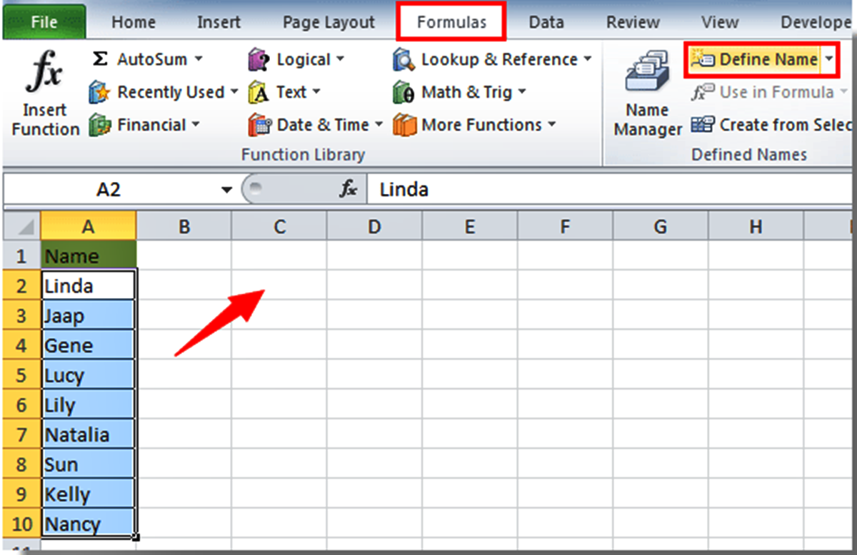
3. Name the Range: Select the range of cells containing the options for the drop-down list. It’s essential to name this range so that it can be easily referenced when setting up the drop-down list. To name the range, go to the Formulas tab, click on the Define Name option, and assign a suitable name to the range.
4. Navigate to the Original Worksheet: Move back to the original worksheet where you want to create the drop-down list.
5. Select the Cell: Choose the cell in which you want the drop-down list to appear. This cell will be the one users can select from when entering data.
6. Data Validation: In the Excel ribbon, navigate to the Data tab and click on Data Validation.
7. Set the Validation Criteria: In the Data Validation dialog box, select “List” as the validation criteria. Under the “Source” field, enter the name of the range that you previously named containing the options for the drop-down list. Make sure to include an equal sign before the range name (e.g., “=RangeName”).
8. Apply the Validation: Click on the “OK” button to apply the data validation to the selected cell, creating the drop-down list.
9. Test the Drop-Down List: To test the functionality of the drop-down list, click on the drop-down arrow in the selected cell. You should see the options from the separate worksheet appear in the drop-down menu. Users can now select an option from the list when entering data into the cell.
By creating a drop-down list in a separate worksheet, you can easily manage and update the list of options without affecting the original worksheet. This enhances the flexibility and organization of your Excel spreadsheet, making it more efficient to work with.
Selecting the Cell for the Drop-Down List
When creating a drop-down list in Excel, it is important to select the appropriate cell where you want the drop-down list to appear. The selected cell will be the one in which users can choose options from the drop-down menu. Follow the steps below to select the cell for the drop-down list:
1. Open the Excel Worksheet: Start by opening the Excel worksheet where you want to create the drop-down list.
2. Navigate to the Desired Cell: Move to the worksheet and navigate to the specific cell where you want the drop-down list to be located. This can be any cell within the worksheet.
3. Determine the Cell Size: Consider the size of the cell to ensure that it can accommodate the drop-down list. If the cell has a small width or height, it may not display the full drop-down list, causing the options to be cut off. Adjust the size of the cell if necessary to ensure sufficient space for the drop-down menu.
4. Single or Multiple Cells: Decide whether you want the drop-down list to appear in a single cell or a range of cells. If you choose a single cell, the drop-down arrow will only appear in that cell. If you select a range of cells, the drop-down arrow will be displayed in each cell within the selected range.
5. Select the Cell or Range: Click on the desired cell or click and drag to select a range of cells where you want the drop-down list to be created. Take note of the selected cell or cell range, as it will be referenced in the next steps.
6. Options Only Visible in the Selected Cell: Keep in mind that the drop-down list options will only be visible in the cell or cells where the drop-down arrow is displayed. Other cells in the worksheet will not show the drop-down list, even if they contain the same formula or are part of the same column or row.
7. Positioning and Layout: Consider the layout and positioning of the cell or cell range within the worksheet. Ensure that it is easily accessible to users and placed where it makes logical sense in relation to the surrounding data.
8. Test the Drop-Down List: To test the functionality of the drop-down list, click on the drop-down arrow in the selected cell or cells. You should see the options for the list appear in the drop-down menu. Users can now select the desired option from the list when entering data into the selected cell or cells.
By carefully selecting the cell or cell range for the drop-down list, you can ensure that it is conveniently located, visible, and easily accessible to users. This helps streamline data entry and enhances the user experience when working with your Excel spreadsheet.
Navigating to the Data Validation Option
In order to create a drop-down list in Excel, you need to navigate to the Data Validation option. Data Validation is a powerful feature in Excel that allows you to set rules and restrictions on data entry. It provides the necessary tools to create drop-down lists, ensuring that users can select options from a predefined list. Follow the steps below to navigate to the Data Validation option:
1. Open the Excel Worksheet: Start by opening the Excel worksheet where you want to create the drop-down list.
2. Select the Cell: Click on the cell where you want the drop-down list to be located. This is the cell where users will be able to select options from the drop-down menu.
3. Navigate to the Data Tab: In the Excel ribbon, locate and click on the “Data” tab. This tab contains various data-related options and features.
4. Click on Data Validation: Within the Data tab, look for the “Data Tools” group. In this group, you’ll find the “Data Validation” button. Click on this button to access the Data Validation options.
5. Data Validation Dialog Box: Clicking on the Data Validation button will open the Data Validation dialog box. This dialog box allows you to set rules and restrictions on the selected cell for data entry.
6. Choose Validation Criteria: In the Data Validation dialog box, you’ll find various tabs containing different types of validation criteria. The most relevant tab for creating a drop-down list is the “Settings” tab.
7. Select the List Option: In the Settings tab, select the “List” option from the drop-down menu under “Allow.” This option specifies that you want to create a drop-down list as the validation criteria for the selected cell.
8. Specify the Source: After selecting the “List” option, you need to specify the source of the list. This can either be a range of cells on the same worksheet or a separate worksheet in the same workbook.
9. Customize the Error Alert (Optional): If desired, you can customize the error alert that appears when an invalid value is entered in the cell. The error alert can display a message and provide options for the user to choose from.
10. Apply the Data Validation: Once you have set the desired options in the Data Validation dialog box, click on the “OK” button to apply the data validation to the selected cell. The drop-down list will now be created in the cell, allowing users to select options from the predefined list.
By navigating to the Data Validation option, you gain access to a powerful set of tools that enable you to create drop-down lists in Excel. This helps to streamline data entry, maintain data integrity, and improve the user experience when working with your Excel spreadsheets.
Setting Up the Drop-Down List
Creating a drop-down list in Excel involves setting up the necessary parameters to define the list’s behavior and appearance. This includes specifying the source of the list and configuring any additional settings. Follow the steps below to set up the drop-down list:
1. Open the Excel Worksheet: Start by opening the Excel worksheet where you want to create the drop-down list.
2. Select the Cell: Click on the cell where you want the drop-down list to be located. This is the cell users will interact with to select options from the drop-down menu.
3. Navigate to the Data Validation Option: To access the Data Validation option, go to the Excel ribbon and click on the “Data” tab. Within this tab, look for the “Data Tools” group and click on the “Data Validation” button. This will open the Data Validation dialog box.
4. Choose the List Option: In the Data Validation dialog box, ensure that the “Settings” tab is selected. Under “Allow,” choose the “List” option from the drop-down menu. This will specify that you want to create a drop-down list as the validation criteria.
5. Specify the Source of the List: After selecting the “List” option, you need to specify the source of the list. There are two options:
- Enter the List Source Manually: If you want to enter the list source manually, type the values directly into the “Source” input box, separating each value with a comma.
- Select the List Source Range: If you have the list of options in a separate range of cells, click the selector button next to the “Source” input box. This will allow you to select the range from which the drop-down list will take its options.
6. Apply the Data Validation: Once you have specified the source of the list, click on the “OK” button to apply the data validation and create the drop-down list. The cell you selected will now display a drop-down arrow that users can click to view and select options from the list.
7. Test the Drop-Down List: Verify that the drop-down list works as expected by clicking on the drop-down arrow in the cell you set up. The options you entered or selected should appear in the drop-down menu, allowing users to choose from them when entering data.
By setting up the drop-down list in Excel, you provide users with a convenient and controlled way to select options from a predefined list. This can help improve data accuracy, ensure consistency, and streamline data entry processes within your Excel spreadsheets.
Specifying the Source of the List
When creating a drop-down list in Excel, it is essential to specify the source of the list. The source determines the options that will appear in the drop-down menu for users to select from. Excel provides two methods for specifying the source of the list – entering the list source manually or selecting the list source range. Follow the steps below to specify the source of the list:
1. Open the Excel Worksheet: Start by opening the Excel worksheet where you want to create the drop-down list.
2. Select the Cell: Click on the cell where you want the drop-down list to be located.
3. Navigate to the Data Validation Option: Go to the Excel ribbon and click on the “Data” tab. In the “Data Tools” group, click on the “Data Validation” button to open the Data Validation dialog box.
4. Choose the List Option: In the Data Validation dialog box, ensure that the “Settings” tab is selected. Under “Allow,” choose the “List” option from the drop-down menu.
5. Specify the List Source Manually: To manually enter the list source, type the values directly into the “Source” input box. Separate each value with a comma. For example, if your list consists of “Apple,” “Banana,” and “Orange,” you would enter “Apple,Banana,Orange” (without quotes).
6. Select the List Source Range: To select the list source range, click on the selector button (small square icon) next to the “Source” input box. This will open the worksheet and allow you to select the range of cells that contain the options for the drop-down list. The selected range will be automatically populated into the “Source” input box.
7. Multiple Columns or Sheets: You can also specify a range of multiple columns or even select a range from a different worksheet. Use the appropriate Excel syntax to indicate the range, such as “Sheet2!A1:A3” for a range in Sheet2.
8. Apply the Data Validation: Once you have specified the source of the list, click on the “OK” button to apply the data validation. The drop-down list will now be created in the selected cell, populated with the options from the specified source.
9. Test the Drop-Down List: Test the functionality of the drop-down list by clicking on the drop-down arrow in the selected cell. The options you entered or selected as the source should be displayed in the drop-down menu, allowing users to choose from them when entering data.
By specifying the source of the list correctly, you ensure that the drop-down list in Excel contains the desired options for users to select from. This provides a user-friendly and efficient way to input data while maintaining consistency and accuracy within your Excel spreadsheets.
Entering the List Source
When creating a drop-down list in Excel, it is crucial to enter the list source accurately. The list source determines the options that will populate the drop-down menu for users to select from. You have two options for entering the list source: manually typing the options or selecting a range of cells containing the options. Follow the steps below to enter the list source:
1. Open the Excel Worksheet: Begin by opening the Excel worksheet where you want to create the drop-down list.
2. Select the Cell: Click on the cell where you want the drop-down list to appear.
3. Navigate to the Data Validation Option: Go to the Excel ribbon and click on the “Data” tab. Within the “Data Tools” group, click on the “Data Validation” button to open the Data Validation dialog box.
4. Choose the List Option: In the Data Validation dialog box, ensure the “Settings” tab is selected. Under the “Allow” section, choose the “List” option from the drop-down menu.
5. Enter the List Source Manually: To manually enter the list source, type each option directly into the “Source” input box. Separate each option with a comma. For example, if you want the list to include “Option 1,” “Option 2,” and “Option 3,” you would enter “Option 1, Option 2, Option 3” (without quotes).
6. Select the List Source Range: If your options are already in a range of cells, click on the selector button (small square icon) next to the “Source” input box. This will allow you to select the range of cells that contains the options for the drop-down list. The range will automatically populate into the “Source” input box.
7. Multiple Columns or Sheets: You can also specify a range that spans multiple columns or even select a range from a different worksheet. Use the appropriate Excel syntax to identify the range, such as “Sheet2!A1:A3” for a range in Sheet2.
8. Apply the Data Validation: Once you have entered the list source accurately, click on the “OK” button to apply the data validation. The drop-down list will now be created in the selected cell, with the options from the specified list source.
9. Test the Drop-Down List: To ensure the drop-down list is functioning correctly, click on the drop-down arrow in the selected cell. The options you entered or selected as the list source should appear in the drop-down menu, allowing users to choose from them when entering data.
By correctly entering the list source, you ensure that the drop-down list contains the desired options for users to select from. This enhances data input accuracy, promotes consistency, and streamlines the data entry process in your Excel spreadsheets.
Applying the Drop-Down List to Other Cells
After creating a drop-down list in Excel, you can easily apply it to multiple cells within the same worksheet. This allows users to select options from the drop-down menu in various cells, ensuring consistency and efficiency in data entry. Follow the steps below to apply the drop-down list to other cells:
1. Open the Excel Worksheet: Begin by opening the Excel worksheet that contains the drop-down list.
2. Select the Original Cell: Click on the cell that contains the drop-down list. This is the cell where users can select options from the drop-down menu.
3. Copy the Cell: Press Ctrl+C (or right-click and select “Copy”) to copy the cell with the drop-down list.
4. Select the Target Cells: Click and drag to select the range of cells where you want to apply the same drop-down list. This range can be adjacent or non-adjacent cells within the worksheet.
5. Paste the Cell Formatting: Right-click on the selected range of cells and choose “Paste Special.” In the Paste Special dialog box, select “Validation” and click on the “OK” button. This will copy the data validation, including the drop-down list, to the target cells.
6. Test the Drop-Down List: To verify that the drop-down list has been applied successfully, click on the drop-down arrow in one of the target cells. The same options from the original drop-down list should appear in the drop-down menu for the new cells.
7. Adjust Cell Range (Optional): If needed, you can adjust the range of cells to which the drop-down list is applied. To do this, select the cells that have the drop-down list, right-click and choose “Data Validation,” and update the range in the “Source” field of the Data Validation dialog box.
8. Save and Distribute the Worksheet: Once you have applied the drop-down list to the desired cells, save the worksheet. You can now distribute the worksheet to others, who can utilize the drop-down list functionality in the designated cells.
By applying the drop-down list to other cells, you extend the functionality and convenience of the list throughout your Excel spreadsheet. This promotes consistent data entry and user-friendly interactions across multiple cells within the worksheet.
Modifying the Drop-Down List
Once you have created a drop-down list in Excel, you may need to modify it to add or remove options, change the order of options, or update the list source. Excel provides simple steps to modify the drop-down list while retaining the data validation settings. Follow the steps below to modify the drop-down list:
1. Open the Excel Worksheet: Begin by opening the Excel worksheet that contains the drop-down list you want to modify.
2. Select the Cell: Click on the cell that contains the drop-down list you want to modify. This is the cell where the drop-down arrow is displayed.
3. Access Data Validation: To access the Data Validation settings, go to the Excel ribbon and click on the “Data” tab. Within the “Data Tools” group, click on the “Data Validation” button to open the Data Validation dialog box.
4. Modify the List Source: In the Data Validation dialog box, make the necessary modifications to the list source. This can involve adding or removing options, changing the order of options, or updating the range of cells that serve as the list source.
5. Update the List Source: After modifying the list source, update the source in the “Source” field of the Data Validation dialog box. This can be done by manually editing the source or selecting a new range of cells as the source.
6. Apply the Changes: Once you have made the modifications and updated the list source, click on the “OK” button to apply the changes to the drop-down list.
7. Test the Modified Drop-Down List: To ensure that the modifications have taken effect, click on the drop-down arrow in the cell. The updated options or changes to the order should now be reflected in the drop-down menu.
8. Adjust Cell Range (Optional): If necessary, you can adjust the range of cells to which the modified drop-down list is applied. To do this, select the cells that have the drop-down list, right-click and choose “Data Validation,” and update the range in the “Source” field of the Data Validation dialog box.
9. Save the Worksheet: Once you are satisfied with the modifications to the drop-down list, save the Excel worksheet to preserve the changes.
By having the ability to modify the drop-down list in Excel, you can easily update and customize the list of options to ensure it aligns with your changing data needs. This flexibility enhances data entry accuracy and user satisfaction with the drop-down functionality.
Removing the Drop-Down List
If you no longer need a drop-down list in your Excel spreadsheet, you can easily remove it. Removing the drop-down list allows you to revert the cell back to regular data entry mode. Follow the steps below to remove the drop-down list:
1. Open the Excel Worksheet: Begin by opening the Excel worksheet that contains the drop-down list you want to remove.
2. Select the Cell: Click on the cell that contains the drop-down list you want to remove. This is the cell with the drop-down arrow displayed.
3. Access Data Validation: To access the Data Validation settings, go to the Excel ribbon and click on the “Data” tab. Within the “Data Tools” group, click on the “Data Validation” button to open the Data Validation dialog box.
4. Remove the Data Validation: In the Data Validation dialog box, navigate to the “Settings” tab. Select the “Any Value” option from the “Allow” drop-down menu. This will remove the data validation settings for the selected cell.
5. Remove the Drop-Down Arrow: After removing the data validation, you will notice that the drop-down arrow is no longer visible in the cell. This indicates that the drop-down list has been removed.
6. Repeat for Multiple Cells: If you have applied the drop-down list to multiple cells and want to remove it from all of them, you can repeat the above steps for each cell.
7. Adjust Cell Range (Optional): If necessary, you can adjust the range of cells from which you removed the drop-down list. To do this, select the cells, right-click and choose “Data Validation,” and update the range in the “Source” field of the Data Validation dialog box.
8. Save the Worksheet: Once you have removed the drop-down list, save the Excel worksheet to finalize the changes.
By removing the drop-down list when it is no longer needed, you can simplify data entry for users and revert to regular input mode. This flexibility allows you to adjust your Excel spreadsheet to meet changing requirements and enhance the efficiency of your data management process.