
Why Change the Order of Operations?
When working with formulas in Excel, you may find yourself needing to change the order of operations. The order of operations determines the sequence in which Excel carries out calculations within a formula. By default, Excel follows the standard order of operations, where calculations inside parentheses are performed first, followed by exponentiation, multiplication and division, and then addition and subtraction.
However, there may be certain situations where you need to modify the order in which Excel performs calculations. This can help you achieve more accurate results or meet specific requirements for your data analysis or modeling.
One common reason for changing the order of operations is to prioritize certain calculations over others. This can be particularly useful when dealing with complex formulas that involve multiple mathematical operations. By rearranging the order in which the calculations are performed, you can ensure that the formula accurately reflects your intended logic.
Another reason to change the order of operations is when you want to override the default behavior of Excel’s built-in functions. Some Excel functions have a fixed order in which they perform calculations. By changing the order of operations, you can control the sequence in which these functions are evaluated within your formulas.
Moreover, changing the order of operations allows you to apply specific calculations before or after other operations. This flexibility can be beneficial when dealing with data transformations or analyzing complex datasets. By strategically modifying the order, you can manipulate the formula to produce the desired results.
Understanding the Order of Operations in Excel Formulas
Before diving into how to change the order of operations in Excel formulas, it’s crucial to have a solid understanding of the default order of operations. Excel follows the standard mathematical conventions, known as PEMDAS (Parentheses, Exponents, Multiplication and Division, Addition and Subtraction).
The order of operations determines the sequence in which Excel evaluates the various components within a formula. This ensures that calculations are performed accurately and consistently.
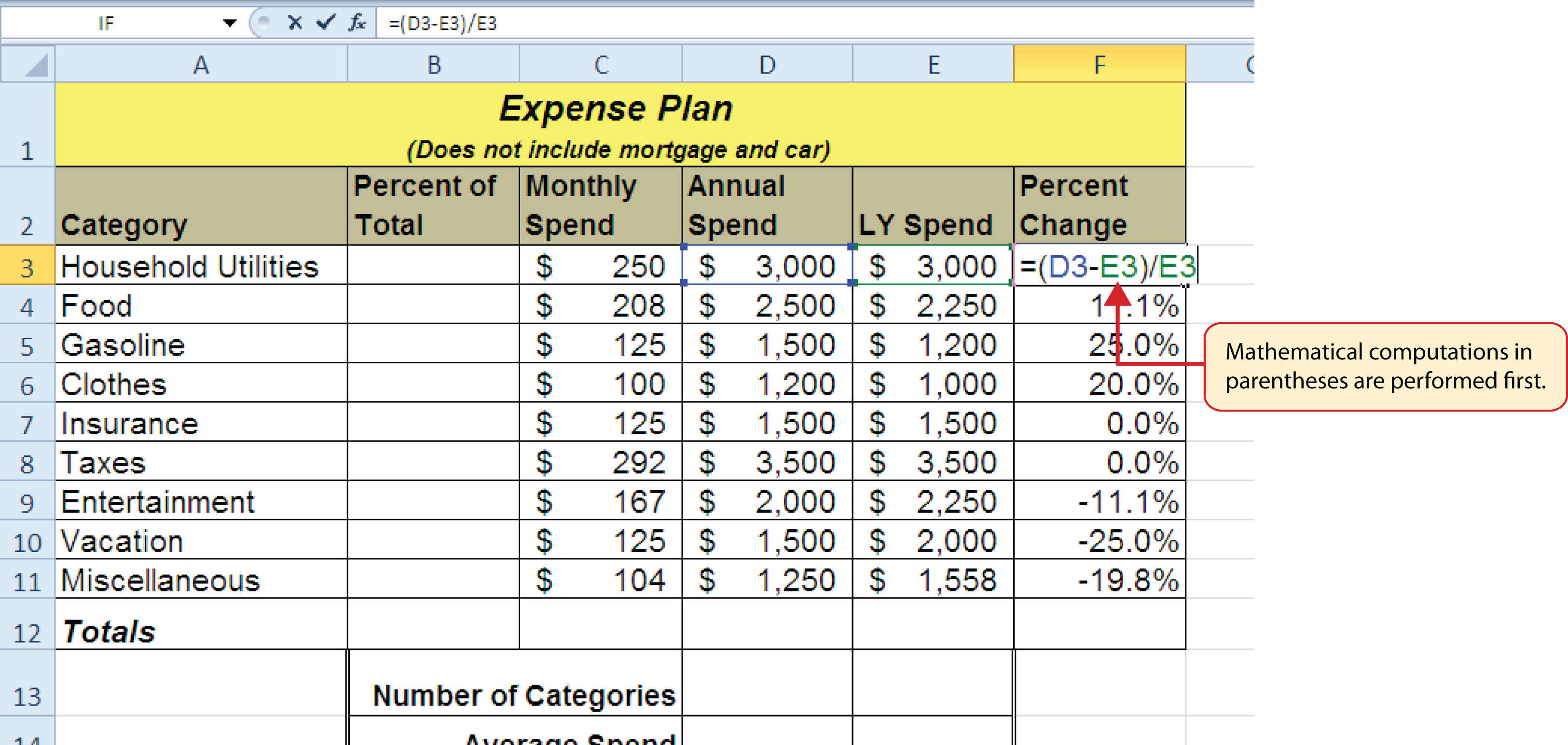
First, Excel prioritizes calculations within parentheses. Any calculations enclosed in parentheses are evaluated first. This allows you to control the order in which calculations should be executed, overriding the default order.
Next, Excel evaluates exponentiation. If any numbers or references in your formula are raised to a power, Excel performs those calculations next.
After that, Excel moves on to multiplication and division operations. In a formula with both multiplication and division, Excel carries out these calculations from left to right.
Finally, Excel performs addition and subtraction operations. Similarly, if a formula includes both addition and subtraction, Excel evaluates them from left to right.
Knowing the order of operations in Excel is crucial for building accurate formulas. If the default order does not align with your desired calculation logic, you can modify the order by using parentheses or built-in functions.
It’s important to note that Excel evaluates formulas from left to right and top to bottom, meaning that if your spreadsheet contains multiple formulas in different cells, Excel will evaluate them in a sequential manner.
By understanding and utilizing the order of operations effectively, you can ensure accurate calculations and optimize your formulas for more complex data analysis tasks in Excel.
Changing the Order of Operations in Excel Formulas
Excel provides several methods for changing the order of operations in formulas. These methods allow you to override the default order and ensure that calculations are carried out according to your specific requirements. Here are some common techniques:
1. Using Parentheses: Adding parentheses to your formulas is the most straightforward way to change the order of operations. By enclosing certain calculations within parentheses, you can make Excel prioritize those calculations over others. For example, if you want Excel to first calculate the sum of two values and then multiply the result by another value, you can use parentheses to group the addition operation.
2. Using Functions: Excel’s built-in functions often have a fixed order in which they perform calculations. By incorporating these functions into your formulas, you can control the order in which they are evaluated. For instance, if you want a specific function to be applied before or after other operations, you can nest it within the formula accordingly.
3. Using Special Functions: Excel also offers specialized functions that can help change the order of operations. The POWER function allows you to raise numbers to a specific power, altering the sequence of calculations. Similarly, the SUM function can be used to group calculations together and modify their order within the formula.
4. Using Logical Functions: In some cases, you may need to change the order of operations based on specific conditions. Excel’s logical functions, such as IF and VLOOKUP, can be used to control the flow of calculations. By incorporating these functions into your formulas, you can conditionally change the order in which certain operations are performed.
5. Using Indirect References: Another technique for changing the order of operations is by using indirect references. The INDIRECT function allows you to create a reference to a cell based on the value in another cell. By dynamically changing the reference, you can alter the order in which calculations are performed, depending on the input value.
6. Using Concatenation: The CONCATENATE function can also be used to change the order of operations. By combining different values or formulas together, you can control the sequence in which calculations are performed. This technique is especially useful when dealing with text or alphanumeric data that requires a specific order of operations.
By utilizing these methods, you can exercise greater control over the order of operations in your Excel formulas. This flexibility allows you to tailor your calculations and achieve more accurate results for your specific data analysis and modeling needs.
Using Parentheses to Change the Order of Operations in Excel Formulas
One of the simplest and most effective ways to change the order of operations in Excel formulas is by using parentheses. By enclosing specific calculations within parentheses, you can prioritize those calculations over others and alter the default order.
To use parentheses, simply place them around the calculations that you want to be performed first. Excel will evaluate the calculations within parentheses before moving on to the remaining operations in the formula.
For example, let’s say you have a formula that involves addition, multiplication, and subtraction. By default, Excel would perform the multiplication first, followed by addition and subtraction. However, if you want to change this order and perform the addition before multiplication, you can use parentheses to group the addition operation. Here’s what the modified formula would look like:
= (A1 + B1) * C1 - D1
In this example, Excel will first calculate the sum of cell A1 and B1 within the parentheses. Then, it will multiply the result by the value in cell C1, and finally, subtract the value in cell D1.
By using parentheses strategically, you can control the order in which calculations are performed within complex formulas. This is particularly useful when you have formulas with multiple mathematical operations and need to prioritize certain calculations over others.
It’s important to note that you can also nest parentheses within one another to create multiple levels of precedence. Excel will evaluate the innermost parentheses first before moving outward.
For example:
= ((A1 + B1) * C1) / (D1 + E1)
In this formula, Excel will first calculate the sum of cell A1 and B1 within the inner parentheses. Then, it will perform the multiplication with the value in cell C1. Finally, it will divide the result by the sum of cell D1 and E1.
By utilizing parentheses to change the order of operations in your Excel formulas, you can customize the calculations to accurately reflect your intended logic and achieve the desired results for your data analysis or modeling tasks.
Using the POWER Function to Change the Order of Operations in Excel Formulas
Excel’s POWER function is a powerful tool that allows you to change the order of operations within your formulas. This function raises a number to a specific power, enabling you to manipulate the sequence of calculations.
To use the POWER function, you need to provide two arguments: the base number and the exponent. The function will then calculate the result by raising the base number to the power of the exponent.
By incorporating the POWER function into your formulas, you can prioritize certain calculations or modify the default order of operations. For example, if you want to perform exponentiation before other mathematical operations, you can use the POWER function to raise a number to a specific power and use the result in your formula.
Let’s consider an example:
= (A1^2) + B1
In this formula, Excel uses the POWER function to square the value in cell A1. The result is then added to the value in cell B1. By using the POWER function, you ensure that the squaring operation is performed first before the addition.
The POWER function becomes particularly valuable when dealing with complex calculations that involve multiple mathematical operations. By strategically applying the POWER function to specific parts of your formula, you can control the order in which calculations are performed and achieve the desired results for your data analysis or modeling requirements.
It’s important to note that you can also use the POWER function with decimal exponents or negative exponents. For example, you can raise a number to the power of 0.5 to calculate the square root, or use a negative exponent to calculate the reciprocal of a number.
For instance:
= (A1^0.5) + B1
In this formula, Excel calculates the square root of the value in cell A1 using the POWER function with an exponent of 0.5. The result is then added to the value in cell B1.
By utilizing the POWER function to change the order of operations in your Excel formulas, you have greater flexibility and control over the sequence in which calculations are performed, allowing you to tailor your formulas to meet your specific needs.
Using the SUM Function to Change the Order of Operations in Excel Formulas
The SUM function in Excel is commonly used to calculate the total sum of a range of cells. However, it can also be leveraged to change the order of operations within your formulas by grouping calculations together.
When you use the SUM function in your formulas, you can prioritize the calculations within the function over other operations in the formula. This can be particularly useful when you want to perform certain calculations before or after other mathematical operations.
To use the SUM function, you need to provide the range of cells you want to sum. Excel will then add up all the values within that range and use the result in your formula.
Let’s consider an example:
= SUM(A1:A5) * B1
In this formula, Excel uses the SUM function to add up the values in cells A1 to A5. The result of the sum is then multiplied by the value in cell B1. By using the SUM function, you ensure that the addition operation takes precedence over the multiplication.
By incorporating the SUM function strategically in your formulas, you can change the order of operations and achieve the desired results for your data analysis or modeling needs.
It’s important to note that you can also combine the SUM function with other functions or mathematical operations within your formulas. This allows you to have even more control over the order of calculations.
For example:
= SUM(A1:A5) / (B1 + C1)
In this formula, Excel uses the SUM function to add up the values in cells A1 to A5. The result is then divided by the sum of the values in cells B1 and C1. By using the SUM function, you ensure that the addition within the function is performed before the division operation.
By utilizing the SUM function to change the order of operations in your Excel formulas, you have greater flexibility and control over the sequence in which calculations are performed, allowing you to tailor your formulas to meet your specific needs.
Using the VLOOKUP Function to Change the Order of Operations in Excel Formulas
The VLOOKUP function is commonly used in Excel to search for a specific value in a vertical lookup table and retrieve a corresponding value from another column. While its primary purpose is to perform lookups, the VLOOKUP function can be utilized to change the order of operations within your formulas.
By incorporating the VLOOKUP function strategically, you can influence the sequence in which calculations are performed and modify the default order of operations.
To use the VLOOKUP function, you need to provide four arguments: the lookup value, the table or range to search, the column index number, and the range lookup option.
Let’s consider an example:
= VLOOKUP(A1, B1:D5, 3, FALSE) + C1
In this formula, the VLOOKUP function searches for the value in cell A1 within the range B1:D5. It then retrieves the corresponding value from the third column and adds it to the value in cell C1.
By using the VLOOKUP function, you can ensure that the lookup and retrieval of values occur before the addition operation.
Furthermore, the VLOOKUP function allows you to conditionally change the order of operations. By utilizing a logical comparison within the function, you can specify when the lookup and retrieval should take place.
For example:
= IF(A1 > 0, VLOOKUP(A1, B1:D5, 3, FALSE), 0)
In this formula, the IF function is used to evaluate whether the value in cell A1 is greater than zero. If it is, the VLOOKUP function performs the lookup and retrieval as defined in the TRUE condition. Otherwise, it returns zero. By incorporating the VLOOKUP function within the IF function, you can control when the lookup operation occurs based on specific conditions.
By strategically utilizing the VLOOKUP function within your Excel formulas, you can change the order of operations and achieve the desired results for your data analysis or modeling requirements. Whether it’s performing lookups or incorporating conditional logic, the VLOOKUP function provides flexibility and control over the sequence of calculations.
Using the IF Function to Change the Order of Operations in Excel Formulas
The IF function in Excel allows you to perform conditional evaluations and change the order of operations within your formulas. This function enables you to alter the sequence in which calculations are performed based on specific conditions or criteria.
The IF function takes three arguments: the logical test, the value_if_true, and the value_if_false. It evaluates the logical test and returns the value_if_true if the test is met, or the value_if_false if the test is not met.
By incorporating the IF function into your formulas, you can determine when certain calculations should be performed, effectively modifying the order of operations.
Let’s consider an example:
= IF(A1 > 0, A1 * B1, 0)
In this formula, the IF function checks if the value in cell A1 is greater than zero. If it is, the formula multiplies the value in cell A1 with the value in cell B1. If the test is not met (i.e., the value in A1 is not greater than zero), the formula returns zero.
By using the IF function, you can control the sequence of calculations by conditionally determining when certain operations should be performed.
The IF function becomes particularly valuable when combined with other functions or mathematical operations within your formulas. It allows you to prioritize specific calculations or manipulate the order of operations based on specific criteria.
For example:
= IF(A1 > 0, SUM(B1:B5), A1 + B1)
In this formula, the IF function checks if the value in cell A1 is greater than zero. If it is, the formula uses the SUM function to add up the values in the range B1:B5. Otherwise, it performs the addition of the values in cells A1 and B1. By using the IF function, you can dynamically change the order of operations based on the condition specified.
By strategically leveraging the IF function within your Excel formulas, you have the flexibility and control to modify the order of operations, ensuring that calculations are performed according to your specific requirements. Whether it’s evaluating conditions or incorporating conditional logic, the IF function is a powerful tool for customizing your formulas.
Using the INDIRECT Function to Change the Order of Operations in Excel Formulas
The INDIRECT function in Excel allows you to dynamically change the order of operations within your formulas by creating references to cells based on the value in another cell. This function enables you to manipulate the sequence in which calculations are performed based on changing input values.
The INDIRECT function takes one argument, which is the cell reference or named range you want to use. The value in the specified cell is then used as the reference for your formula.
By incorporating the INDIRECT function into your formulas, you can alter the order of operations and determine which calculations are executed first.
Let’s consider an example:
= INDIRECT("A" & A1) + B1
In this formula, the INDIRECT function creates a reference to cell A1 by concatenating the letter “A” with the value in cell A1. The result is then added to the value in cell B1. The INDIRECT function dynamically changes the reference based on the value in A1, allowing you to change the order of operations based on the input value.
The INDIRECT function becomes particularly useful when combined with other mathematical operations or functions in your formulas. It allows you to prioritize calculations or dynamically adjust the sequence of operations.
For example:
= INDIRECT("A" & A1) * (C1 + D1)
In this formula, the INDIRECT function creates a reference to cell A1 by concatenating the letter “A” with the value in cell A1. The result is then multiplied by the sum of the values in cells C1 and D1. By using the INDIRECT function, you can dynamically change the order of operations based on the input value in A1.
By strategically utilizing the INDIRECT function within your Excel formulas, you have the flexibility and control to modify the order of operations based on changing input values. This allows you to adapt your calculations to meet your specific needs and achieve the desired results in your data analysis or modeling tasks.
Using the CONCATENATE Function to Change the Order of Operations in Excel Formulas
The CONCATENATE function in Excel allows you to manipulate the order of operations within your formulas by combining different values or formulas together. This function enables you to control the sequence in which calculations are performed by customizing the order of the concatenated elements.
The CONCATENATE function takes multiple arguments, which can be text strings, numbers, or references. It concatenates these elements and returns the combined result as a single text string.
By incorporating the CONCATENATE function into your formulas, you can change the order of operations and determine when certain calculations are executed.
Let’s consider an example:
= CONCATENATE(A1, B1) * C1
In this formula, the CONCATENATE function combines the values in cells A1 and B1 into a single text string. The result is then multiplied by the value in cell C1. By using the CONCATENATE function, you can ensure that the concatenation is performed before the multiplication.
The CONCATENATE function becomes particularly valuable when combined with other functions or mathematical operations within your formulas. It allows you to prioritize specific calculations or manipulate the order of operations based on your requirements.
For example:
= CONCATENATE("Total: ", SUM(A1:A5), " units") / B1
In this formula, the CONCATENATE function combines the text “Total: “, the sum of the values in the range A1:A5, and the text ” units” into a single text string. The result is then divided by the value in cell B1. By using the CONCATENATE function, you can dynamically change the order of operations based on the concatenation sequence.
By strategically utilizing the CONCATENATE function within your Excel formulas, you have the flexibility and control to modify the order of operations and customize the calculations according to your specific needs. Whether it’s combining text strings or incorporating numeric values, the CONCATENATE function provides a powerful way to manipulate the order of operations within your formulas.