
Basics of Conditional Formatting in Excel
Conditional formatting is a powerful feature in Microsoft Excel that allows you to highlight cells or ranges of cells based on specific criteria. It is a handy tool that helps you visually analyze data, spot trends, and identify outliers without the need for complex formulas or manual formatting. In this section, we will explore the basics of conditional formatting and how to get started with it.
To apply conditional formatting in Excel, start by selecting the cells or range of cells you want to format. Then, go to the ‘Home’ tab on the Excel ribbon and click on the ‘Conditional Formatting’ button. A drop-down menu will appear with various formatting options.
You can choose from a range of predefined formatting rules, such as highlighting cells that contain specific text or values, using data bars to represent values, or adding color scales to visualize data ranges. These predefined rules are quick and easy to apply, making them suitable for simple formatting needs.
However, if you require more advanced formatting options, you can create custom rules using formulas. Excel allows you to define your own criteria based on formulas that evaluate the cell values. This opens up a whole new level of flexibility and control over your conditional formatting.
The ‘New Formatting Rule’ dialog box provides a formula input bar where you can enter your formula. Excel will evaluate the formula for each selected cell, and if it returns true, the formatting rule will be applied to that cell.
For example, let’s say you have a list of sales figures in column A, and you want to highlight cells that exceed a certain threshold. You can use the formula ‘=$A1>5000’ to check if the value in cell A1 is greater than 5000. If the formula evaluates to true, you can specify a formatting style, such as bold font or a red fill, to visually highlight the cell.
Conditional formatting formulas can be as simple or as complex as you need them to be. You can incorporate logical operators, comparison operators, and even functions to create intricate formatting rules that suit your specific requirements.
Understanding Formulas in Conditional Formatting
When it comes to conditional formatting in Excel, formulas play a crucial role in determining which cells should be formatted and how they should be formatted. Understanding how formulas work in conditional formatting is essential to utilize this feature effectively. In this section, let’s delve deeper into the world of conditional formatting formulas.
Formulas in conditional formatting are similar to regular Excel formulas but with a slight difference. Instead of returning a value, these formulas evaluate to either true or false. If a formula evaluates to true for a particular cell or range, the formatting rule associated with that formula will be applied to the cell(s).
You can use comparison operators, logical operators, and functions to create powerful and dynamic formulas. Comparison operators such as greater than (>), less than (<), equal to (=), and not equal to (<>), allow you to compare cell values and set specific formatting rules based on these comparisons.
Logical operators, such as AND, OR, and NOT, help you combine multiple conditions in a single formula. For instance, you might want to highlight cells where the value is greater than 10 AND less than 20. In this case, you can use the AND operator in your formula to check both conditions simultaneously.
Functions in conditional formatting formulas allow you to apply complex formatting rules based on calculations and analyses. Excel offers a wide range of functions that you can leverage in your formulas, such as SUM, AVERAGE, COUNT, and IF. These functions add a dynamic aspect to your conditional formatting by considering specific ranges or cell values in your calculations.
One important consideration when using formulas in conditional formatting is the use of cell references. By referencing other cells in your formula, you can create dynamic formatting rules that adapt to changes in your data. For example, you can highlight cells that are greater than the average of a range by referencing the average cell in your formula.
It’s worth noting that conditional formatting formulas can become quite complex, especially when dealing with large datasets or multiple conditions. In such cases, it’s important to troubleshoot your formulas if the formatting doesn’t work as expected. Double-check syntax and ensure that cell references are correct.
Understanding the fundamentals of conditional formatting formulas will help you unlock the full potential of this feature. By combining operators, functions, and cell references effectively, you can create sophisticated formatting rules that make your data more visually appealing and insightful.
Creating Simple Rules with Formulas
Conditional formatting in Excel allows you to create simple rules using formulas to highlight cells based on specific criteria. These rules can be helpful in drawing attention to important data points, identifying trends, or spotting errors. In this section, we will explore how to create simple formatting rules using formulas in Excel.
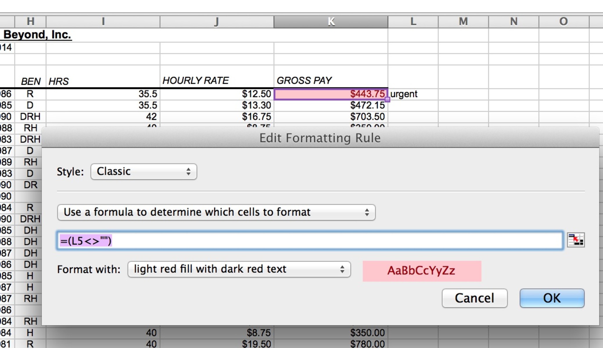
To create a simple rule with a formula, start by selecting the cells or range of cells you want to format. Then, navigate to the ‘Conditional Formatting’ button in the ‘Home’ tab on the Excel ribbon and choose ‘New Rule’. In the ‘New Formatting Rule’ dialog box, select the option ‘Use a formula to determine which cells to format’.
In the formula input bar, you can enter your formula that evaluates to either true or false. If the formula returns true for a particular cell, the formatting rule will be applied to that cell. Let’s walk through an example to illustrate this.
Suppose you have a list of temperatures in column A, and you want to highlight all the temperatures that exceed 80 degrees Fahrenheit. You can create a simple formatting rule using the formula ‘=A1>80’. This formula checks if the value in cell A1 is greater than 80 and applies the formatting rule if the condition is met.
Additionally, you can specify the formatting style to be applied to the selected cells. You can choose from options such as font color, background color, bold, italics, underline, and more. This allows you to easily visualize and distinguish the cells that meet your specified condition.
Creating simple rules with formulas enables you to customize the formatting based on your specific requirements. For instance, you can highlight cells with negative values using the formula ‘A1<0', or you can emphasize dates that fall within a particular range using the formula 'AND(A1>=DATE(2022,1,1), A1<=DATE(2022,12,31))'.
Remember to use appropriate comparison operators, such as greater than (>), less than (<), equal to (=), or not equal to (<>), depending on the desired condition you wish to apply. You can also combine conditions using logical operators ‘AND’ and ‘OR’, allowing for more complex formatting rules.
Simple rules with formulas provide a versatile way to highlight, emphasize, or visually represent specific conditions in your data. Experiment with different formulas and formatting options to make your data more visually appealing and easier to interpret.
Using Comparison Operators in Formulas
When creating conditional formatting rules in Excel, comparison operators play a crucial role in evaluating cell values and applying the desired formatting. These operators allow you to compare values and make decisions based on the results. In this section, we will explore the different comparison operators you can use in formulas for conditional formatting.
Excel provides a variety of comparison operators that you can use in your conditional formatting formulas. These operators include:
- Greater than (>): This operator checks if a value is greater than another value. For example, the formula ‘=A1>10’ highlights cells where the value in cell A1 is greater than 10.
- Less than (<): This operator checks if a value is less than another value. For instance, '=B1<50' will highlight cells where the value in cell B1 is less than 50.
- Equal to (=): This operator checks if a value is equal to another value. ‘=C1=100’ will highlight cells where the value in cell C1 is equal to 100.
- Not equal to (<>): This operator checks if a value is not equal to another value. For example, the formula ‘=D1<>0′ will highlight cells where the value in cell D1 is not equal to zero.
- Greater than or equal to (>=): This operator checks if a value is greater than or equal to another value. ‘=E1>=20’ will highlight cells where the value in cell E1 is greater than or equal to 20.
- Less than or equal to (<=): This operator checks if a value is less than or equal to another value. '=F1<=5' will highlight cells where the value in cell F1 is less than or equal to 5.
Using these comparison operators opens up various possibilities for conditional formatting. You can combine them with other elements in your formulas, such as cell references or functions, to create advanced formatting rules.
For example, you can use comparison operators to highlight sales figures that exceed a specific threshold, identify the highest or lowest values in a range, or flag values that are significantly different from the average.
It’s important to remember that comparison operators should be used in the context of the particular condition you want to apply. Ensure that the cell references and values in your formulas match the desired comparison criteria.
By utilizing comparison operators effectively in conditional formatting formulas, you can highlight specific data points based on their relationships with other values. This allows for better data analysis and visual representation to identify patterns, trends, and outliers in your Excel worksheets.
Using Logical Operators in Formulas
Logical operators are essential components when creating complex conditional formatting rules in Excel. These operators allow you to combine multiple conditions and make more sophisticated decisions based on the results. In this section, we will explore the various logical operators you can use in formulas for conditional formatting.
Excel offers three main logical operators that you can use in your conditional formatting formulas:
- AND: This operator allows you to combine multiple conditions, and all conditions must be true for the formula to evaluate as true. For example, the formula ‘=AND(A1>10, B1<20)' will highlight cells where the value in cell A1 is greater than 10 and the value in cell B1 is less than 20.
- OR: This operator allows you to combine multiple conditions, and at least one condition must be true for the formula to evaluate as true. For instance, the formula ‘=OR(C1=”Red”, C1=”Blue”)’ will highlight cells where the value in cell C1 is either “Red” or “Blue”.
- NOT: This operator negates the result of a condition. It returns true if the condition is false and false if the condition is true. For example, the formula ‘=NOT(D1>50)’ will highlight cells where the value in cell D1 is not greater than 50.
Using logical operators allows you to create conditional formatting rules that consider multiple criteria simultaneously. This enables you to apply formatting based on more complex conditions and make your formatting rules more precise.
For example, you can combine logical operators with comparison operators to highlight cells that meet specific conditions. You can use logical AND to highlight cells where one value is greater than 10 and another value is less than 20. Similarly, you can use logical OR to highlight cells where the value is either “Red” or “Blue”.
It’s important to be mindful of the order of operations when using logical operators in formulas. The Excel formula calculation order follows the principle of parentheses first, then NOT, followed by AND, and finally OR. If necessary, you can use parentheses to control the order of evaluation and ensure your formula works as intended.
By utilizing logical operators effectively in your conditional formatting formulas, you can create more intricate rules and customize the formatting based on multiple conditions. This helps you gain deeper insights into your data and visually represent complex relationships within your Excel worksheets.
Combining Multiple Conditions in a Formula
When working with conditional formatting in Excel, you may often find the need to combine multiple conditions to create more advanced and specific formatting rules. Excel provides several techniques to combine multiple conditions in a formula to achieve the desired result. In this section, we will explore how to combine multiple conditions in a formula for conditional formatting.
Excel allows you to combine conditions in a formula using logical operators such as AND and OR. These operators enable you to create complex rules by evaluating multiple conditions simultaneously.
Let’s consider an example where you want to highlight cells in a sales data range where both the salesperson is “John” and the sales amount is greater than $1000. In this case, you can use the AND operator to combine these conditions in a formula:
=AND(A1="John", B1>1000)
In this formula, the AND operator ensures that both conditions, A1 being equal to “John” and B1 being greater than 1000, are met for the formula to evaluate as true. If both conditions are satisfied, the formatting rule associated with the formula will be applied to the cell.
If, on the other hand, you want to highlight cells where either the salesperson is “John” or the sales amount is greater than $1000, you can use the OR operator:
=OR(A1="John", B1>1000)
In this formula, the OR operator allows for either condition to be true for the formula to evaluate as true. If either condition is satisfied, the formatting rule associated with the formula will be applied to the cell.
It’s important to note that you can nest logical operators within each other to create more complex conditions. You can use parentheses to group conditions, establishing the order of evaluation and ensuring that your formula produces accurate results.
For example, if you want to highlight cells where the salesperson is “John” and the sales amount is either greater than $1000 or less than $100, you can use the following formula:
=AND(A1="John", OR(B1>1000, B1<100))
In this formula, the OR operator is nested within the AND operator, allowing for different combinations of true/false evaluations to meet the overall condition.
By combining multiple conditions in a formula, you can create intricate and precise rules for conditional formatting. This allows you to highlight cells based on complex relationships and criteria within your Excel data.
Using Cell References in Formulas
When working with conditional formatting in Excel, using cell references in formulas allows you to create dynamic and adaptable formatting rules. Cell references enable your formulas to refer to the values in other cells, making your conditional formatting rules flexible and responsive to changes in the data. In this section, we will explore the benefits and techniques of using cell references in formulas for conditional formatting.
Using cell references in conditional formatting formulas allows you to create formatting rules that can be automatically applied to multiple cells in your worksheet. This eliminates the need to manually adjust the formulas for each cell, saving you time and effort.
To use a cell reference, simply replace a specific value in your formula with the reference to the cell containing the value. This way, whenever the referenced cell changes, the formula will automatically adjust and apply the formatting accordingly.
For example, suppose you have a range of cells containing sales data, and you want to highlight cells that exceed the average sales. Instead of manually entering the average value into your formula, you can use a cell reference to refer to the cell where the average value is calculated.
The formula could be something like:
=A1>$D$1
In this formula, $D$1 is the cell reference to the cell containing the average value. By using the dollar sign before the column letter and row number, we create an absolute reference, which means the reference will not change when copied or applied to other cells. This ensures that the formula consistently refers to the desired cell.
On the other hand, if you want to create a relative reference, which adjusts when copied or applied to other cells, you can use cell references without the dollar sign. For example, if you want to highlight cells that are greater than the value in the cell one column to the left, you can use the formula:
=A1>A1-1
In this formula, A1 is the cell reference to the current cell, and A1-1 is the reference to the cell one column to the left. As you copy or apply this formula to other cells, the references will adjust accordingly, always referring to the respective cell relative to the current cell.
Using cell references in conditional formatting formulas allows for more dynamic and adaptable rules. You can easily extend the formatting to a larger range of cells, and the formulas will automatically adjust to the values in each cell. This flexibility makes your conditional formatting more efficient and scalable.
By harnessing the power of cell references, you can create conditional formatting rules that respond to changes in your data and provide meaningful insights into your Excel worksheets.
Working with Relative and Absolute Cell References
When using cell references in conditional formatting formulas, understanding the distinction between relative and absolute references is crucial. Relative references adjust their position when copied or applied to other cells, while absolute references remain fixed regardless of their location. In this section, we will explore the benefits and techniques of working with relative and absolute cell references in conditional formatting.
Relative references are the default type of cell reference in Excel. When you create a formula with a relative reference, the reference adjusts automatically when copied or applied to other cells. This means that the formula will always refer to the cell that is a certain number of rows or columns away from the current cell.
For example, if you have a formatting rule that highlights cells greater than the value in the cell to the left, you can use the formula:
=A1>A1-1
In this formula, the cell references A1 and A1-1 are relative references. When you copy or apply this formula to other cells, Excel adjusts the references accordingly. For example, if you apply the formula to cell B2, it will become =B2>B2-1, referring to the value in the cell one column to the left of the current cell.
On the other hand, absolute references are used when you need a reference to remain fixed, regardless of its position. This is achieved by adding dollar signs ($) before the column letter and row number of the reference. Absolute references do not change when copied or applied to other cells.
For example, if you have a formatting rule that highlights cells greater than a specific threshold value, you can use an absolute reference to ensure the threshold value remains constant:
=A1>$D$1
In this formula, $D$1 is an absolute reference. When copied or applied to other cells, the formula will always refer to cell D1 for comparison. This is useful when you want to compare all cells in a range to the same fixed value.
It's worth noting that you can also use a mixed reference, which combines relative and absolute components. For example, if you want to keep the column fixed but allow the row to adjust, you can use the formula:
=A1>$D1
In this formula, $D1 is a mixed reference. As the formula is copied or applied to other cells horizontally, the column will stay fixed at D, but the row will adjust accordingly.
Understanding how to work with relative and absolute cell references allows you to create more flexible and versatile conditional formatting rules. By adjusting references dynamically or keeping them fixed, you can tailor your formatting based on specific needs and effectively analyze your Excel data.
Troubleshooting Formulas in Conditional Formatting
While creating conditional formatting rules in Excel, it is common to encounter issues or unexpected results in your formulas. Troubleshooting these formulas is an essential skill to ensure that your conditional formatting works as intended. In this section, we will explore some common troubleshooting techniques to help you identify and resolve issues with formulas in conditional formatting.
1. Check syntax: The first step in troubleshooting any formula is to review its syntax carefully. Ensure that all brackets, commas, and quotation marks are correctly placed and that the formula follows the syntax rules of Excel. Even a minor syntax error can cause the formula to malfunction. If you're uncertain about the correct syntax, consult Excel's documentation or use the formula builder tool.
2. Verify cell references: One of the common issues in conditional formatting formulas is referencing the wrong cell or range. Double-check that the cell references in your formulas are accurate and correctly match the data you want to evaluate. Additionally, check if the cell references are relative, absolute, or mixed, as this can impact how the formula behaves when copied to other cells.
3. Debug step by step: If your formula is complex, consider breaking it down into smaller components and evaluating each part individually. This can help pinpoint the source of the problem. You can use Excel's formula auditing tools, such as the evaluate formula feature, to step through the formula and identify any errors or unexpected results at each stage.
4. Confirm data types: Ensure that the cell values you are comparing in your formulas have the correct data types. For example, if you are comparing text, make sure you enclose the text in quotation marks. Excel may interpret numbers, dates, or text differently, which can lead to formula errors or unexpected results.
5. Consider calculation order: Conditional formatting formulas follow Excel's calculation order. If you have formulas that refer to other cells or include functions, ensure that the referenced cells are calculated before the conditional formatting rules are evaluated. You can adjust the calculation order using parentheses or by rearranging your formulas.
6. Test with sample data: If you're still encountering issues, try testing your conditional formatting formulas with sample data. Create a small sample range that includes various scenarios you want to highlight or format, and then apply your formula to see if it produces the expected results. This can help identify any specific patterns or outliers that may be causing issues.
Remember that troubleshooting formulas in conditional formatting may require some trial and error. Make small adjustments to your formulas, test them, and analyze the results until you achieve the desired outcome.
By utilizing these troubleshooting techniques, you can effectively address formula issues in conditional formatting and ensure that your formatting rules accurately represent and highlight the desired conditions in your Excel worksheets.
Using Conditional Formatting Formulas with Functions
Conditional formatting in Excel becomes even more powerful when you combine it with functions. Functions allow you to perform calculations, manipulate data, and apply complex logic in your conditional formatting formulas. In this section, we will explore how to use functions effectively in conditional formatting to create dynamic and customized formatting rules.
Excel offers a wide range of functions that you can use in your conditional formatting formulas. These functions can help you analyze data, calculate averages, count occurrences, and perform various other operations. By incorporating functions into your conditional formatting formulas, you can create formatting rules that go beyond simple comparisons and take into account more complex criteria.
For example, let's say you have a sales data range, and you want to highlight cells where the sales amount is above the average. You can use the AVERAGE function to calculate the average value, and then compare each cell to this average using a conditional formatting formula.
The formula could be something like:
=A1>AVERAGE(A:A)
In this formula, AVERAGE(A:A) is a function that calculates the average of all the values in column A. The formula compares each cell (starting from A1 in this case) to the calculated average, and if the cell value is greater, the formatting rule is applied.
Functions can also be used to format based on specific conditions or patterns in your data. For instance, you can use the MOD function to highlight cells that contain even numbers:
=MOD(A1,2)=0
In this formula, the MOD function calculates the remainder when dividing the value in cell A1 by 2. If the remainder is 0 (indicating an even number), the formatting rule is applied to the cell.
Furthermore, you can combine functions with other operators, such as comparison operators and logical operators, to create more complex rules. You can use functions like SUM, MAX, MIN, COUNT, IF, and many more to perform calculations and analyze data within your conditional formatting rules.
When working with functions in conditional formatting, it's essential to consider relative and absolute cell references, as well as the calculation order of your formulas. These factors can affect how the functions interpret and calculate the values correctly.
By leveraging the power of functions in your conditional formatting formulas, you can create rules that adapt to changes in your data, perform custom calculations, and highlight patterns or outliers. This enables you to gain deeper insights into your Excel worksheets and present data in a more meaningful and visually appealing way.
Examples of Advanced Conditional Formatting Formulas
Conditional formatting in Excel offers a wide range of possibilities for creating advanced and customized formatting rules. By combining operators, functions, and cell references, you can create intricate formulas that highlight specific conditions, patterns, or outliers in your data. In this section, we will explore some examples of advanced conditional formatting formulas to showcase the versatility and power of this feature.
Example 1: Highlighting Top Performers
Suppose you have a range of sales data, and you want to highlight the top 10% of performers. You can achieve this by using the PERCENTILE function in your conditional formatting formula:
=A1>=PERCENTILE(A:A, 90%)
In this formula, PERCENTILE(A:A, 90%) calculates the value that represents the top 10% of the data in column A. The formula compares each cell to this calculated value, and if the cell value is greater or equal, the formatting rule is applied.
Example 2: Applying Color Scales
You can use conditional formatting to visually represent data ranges using color scales. For instance, you can apply a color scale that represents the distribution of values across a range. Let's say you have a range of temperatures, and you want to apply a color scale from blue (low) to red (high). You can use the MIN and MAX functions in your conditional formatting formula:
=((A1-MIN(A:A))/(MAX(A:A)-MIN(A:A)))
This formula calculates the normalized value of each cell in relation to the minimum and maximum values in the range. The color scale is then applied based on this normalized value, providing a visual representation of the temperature distribution.
Example 3: Emphasizing Incomplete Tasks
Conditional formatting can also be used to highlight incomplete tasks in a to-do list. Let's assume you have a range of task statuses, with "Complete" and "Incomplete" as the possible values. You can use the EXACT function to compare the cell value to "Incomplete" in your formula:
=EXACT($B1,"Incomplete")
In this formula, $B1 represents an absolute cell reference to the column where the task statuses are located. The formula checks if the value in each cell is exactly equal to "Incomplete", and if so, applies the formatting rule.
These examples provide just a glimpse of the advanced conditional formatting formulas you can create in Excel. By combining different operators, functions, and referencing techniques, you can tailor your formatting rules to meet specific requirements and gain valuable insights from your data.
Tips and Tricks for Using Formulas in Conditional Formatting
Using formulas in conditional formatting allows you to customize and optimize your formatting rules in Excel. To help you make the most out of this feature, here are some tips and tricks to consider when working with formulas in conditional formatting:
1. Experiment and test: Don't be afraid to try different formulas and formatting options to achieve the desired result. Experimentation is key to finding the right combination that best highlights your data.
2. Use descriptive cell references: When creating formulas, use cell references that clearly indicate the purpose or data being evaluated. This makes your formulas more readable and easier to understand, especially for others who may work with your spreadsheet.
3. Order your rules: If you have multiple conditional formatting rules, consider the order in which they are applied. Rules are evaluated from top to bottom, so the order matters. Make sure to order the rules in a way that prioritizes the most important conditions.
4. Apply formatting to the entire range: If you want formatting to be applied to a range of cells, apply the conditional formatting rule to the entire range instead of a single cell. This ensures that the formatting is consistent throughout the range, even if the formula references different cells within that range.
5. Use the formula builder: If you're unsure of the correct syntax or need assistance with functions, utilize Excel's formula builder. It provides a user-friendly interface that helps you construct and validate your formulas.
6. Consider performance: Complex and resource-intensive formulas may slow down the responsiveness of your worksheet, especially when applied to large ranges. Try to strike a balance between sophisticated rules and efficient performance.
7. Document your formulas: If your conditional formatting formulas are complex or involve multiple conditions, consider adding comments or documentation to explain the logic. This helps you and others understand and maintain the formulas in the future.
8. Reuse and modify existing rules: Don't hesitate to repurpose existing conditional formatting rules for similar scenarios. You can copy and modify existing rules to save time and maintain a consistent formatting approach.
9. Consider conditional formatting precedence: Conditional formatting rules can overlap or conflict with each other. Familiarize yourself with the precedence rules in Excel, where the last applied rule takes precedence. Adjust the order and structure of your rules to avoid conflicts and ensure the desired formatting is applied.
10. Regularly review and update: As your data changes or new requirements arise, periodically review and update your conditional formatting rules to keep them relevant and effective.
By leveraging these tips and tricks, you can harness the full potential of formulas in conditional formatting. This will enable you to create dynamic, insightful, and visually appealing formatting rules in Excel.