
Different ways to highlight data in Excel
Excel offers various methods to highlight data, allowing users to easily identify important information within their spreadsheets. Whether you want to emphasize certain values, spot trends, or track duplicates, Excel’s built-in features provide flexible ways to achieve your goals. Here are some of the different ways you can highlight data in Excel:
1. Conditional formatting: This powerful tool allows you to automatically format cells based on specific conditions. You can highlight cells based on their values, such as highlighting cells with values above or below a certain threshold. Conditional formatting is ideal for visualizing data trends and making it easier to analyze large datasets.
2. Color scales: Color scales are a great way to represent data gradients visually. Excel offers different color scales, such as green-yellow-red, to highlight high and low values in your dataset. This feature is particularly useful when you want to compare values across a range and quickly identify the highest and lowest values.
3. Icon sets: Icon sets add visual icons to your cells to represent different conditions. For example, you can use arrows or smiley faces to indicate whether a value is increasing, decreasing, or staying the same. This method is helpful when you want to present data with a clear visual representation.
4. Highlighting duplicates: Excel allows you to highlight duplicate values within a range. By using the conditional formatting feature, you can easily spot any duplicate entries in your dataset. This is especially useful for data validation purposes or when dealing with large datasets where duplicates can be easily overlooked.
5. Data bars: Data bars are horizontal bars within cells that visually represent the values they contain. The length of the bar varies based on the value it represents. This method helps you quickly gauge and compare values within a range.
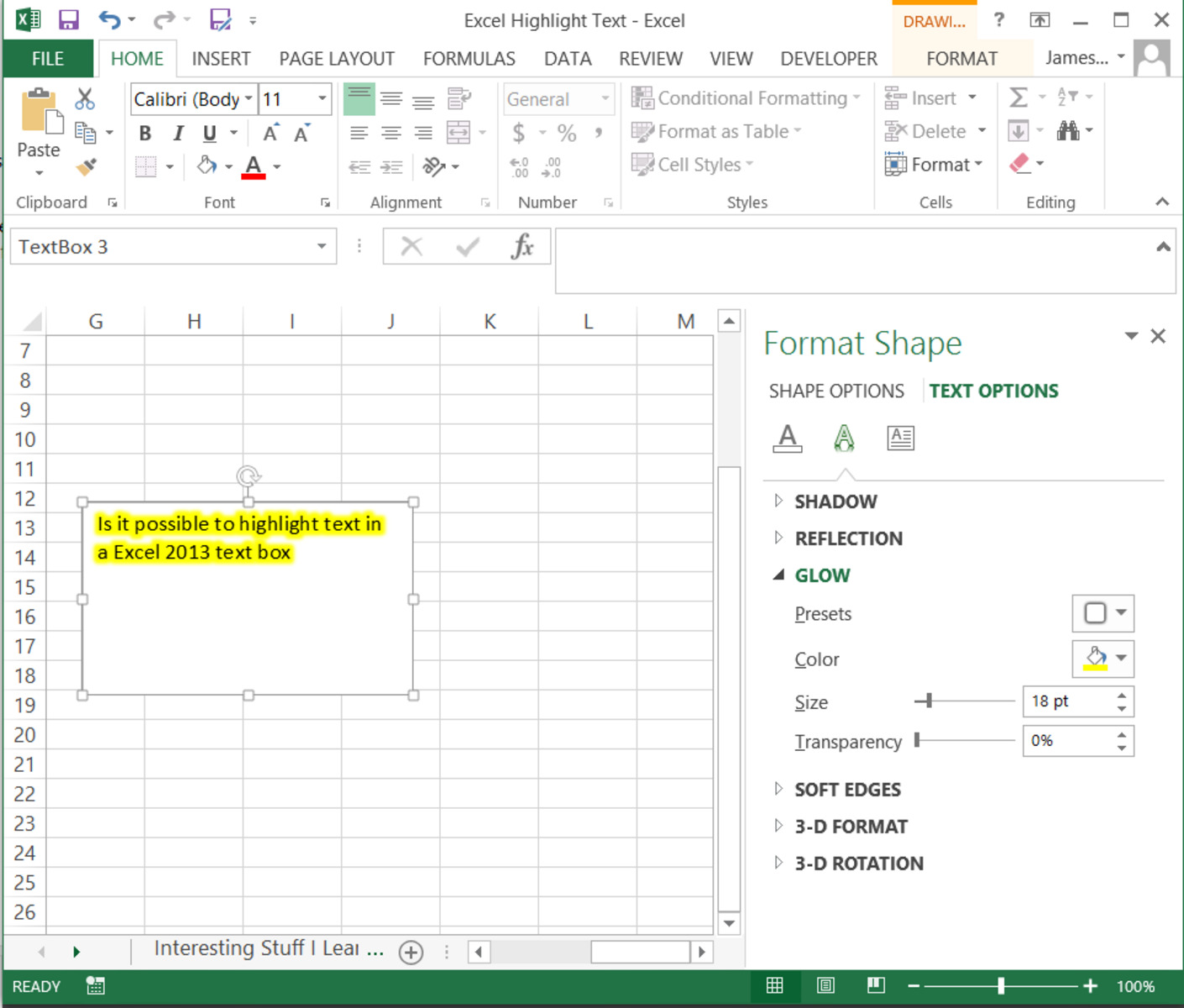
6. Text highlighting: You can also highlight specific text within cells to draw attention to specific phrases or keywords. Excel provides formatting options to change the color or style of the selected text for emphasis.
7. Formula-based highlighting: Excel allows you to create custom formulas to highlight cells based on specific criteria. This gives you more control over the highlighting process and allows for complex conditions to be met before formatting is applied.
These are just a few of the different ways you can highlight data in Excel. By utilizing these features, you can enhance the visual presentation of your spreadsheets and make it easier to interpret and analyze your data.
Using conditional formatting to highlight data in Excel
Conditional formatting is a powerful feature in Excel that allows you to automatically apply formatting to cells based on specific criteria or conditions. This makes it easy to highlight important data and draw attention to specific trends or patterns within your spreadsheet. Here’s how you can use conditional formatting to highlight data in Excel:
Formatting cells based on their values: With conditional formatting, you can highlight cells based on their values. For example, you can set up a rule to highlight all cells that contain a certain number or text. This can be helpful when you want to quickly identify specific data points in your spreadsheet.
Highlighting cells that meet specific criteria: Conditional formatting allows you to specify specific criteria to highlight cells. For instance, you can highlight all cells that are greater than a certain value or those that are within a certain date range. This feature is helpful for flagging outliers or focusing on specific subsets of data.
Creating custom rules for conditional formatting: Excel offers predefined rules for conditional formatting, but you can also create custom rules to suit your specific needs. You can combine multiple criteria or use complex formulas to highlight data. This gives you more flexibility in determining which data to highlight and how to format it.
Using color scales to highlight data: Color scales allow you to apply different colors to cells based on their values within a range. This makes it easier to visually identify high and low values or see trends at a glance. Excel provides a range of color scales to choose from, and you can customize them to fit your preferences or specific requirements.
Using icon sets to highlight data: You can utilize icon sets to visually represent data within your spreadsheet. These icons can represent different conditions, such as arrows indicating an increase or decrease in values, or symbols denoting specific categories. This makes it easy to highlight trends or compare data visually.
Highlighting duplicate values: Excel’s conditional formatting feature allows you to highlight duplicate values within a range. This can be particularly useful when dealing with large datasets or when you need to ensure data accuracy. By flagging duplicate entries, you can quickly identify and address any inconsistencies or errors in your data.
Conditional formatting in Excel provides a range of options to highlight and emphasize data within your spreadsheets. By utilizing these features effectively, you can make your data more visually appealing, facilitate data analysis, and improve decision-making based on the highlighted information.
Formatting cells based on their values
Formatting cells based on their values is a useful feature in Excel’s conditional formatting tool. This allows you to automatically apply formatting options, such as font color, fill color, or borders, to cells that meet specific criteria. By highlighting cells with certain values, you can draw attention to important data points and make your spreadsheet more visually appealing. Here’s how you can format cells based on their values in Excel:
1. Highlight cells containing specific values: One way to format cells based on their values is to highlight cells that contain specific values. For example, you can apply formatting to cells that contain values greater than a certain number or cells that contain specific text. This is useful when you want to emphasize specific data points or identify outliers.
2. Formatting cells based on numerical ranges: You can also format cells based on numerical ranges. For instance, you can set up conditional formatting rules to highlight cells with values within a certain range, such as cells that fall between 50 and 100. This makes it easy to identify data within specific thresholds or categories.
3. Formatting cells based on date ranges: If you’re working with dates, you can format cells based on date ranges. For example, you can use conditional formatting to highlight cells that contain dates within the past week or cells that fall within a specific month. This is particularly helpful when analyzing time-sensitive data or tracking progress over time.
4. Formatting cells based on text conditions: Conditional formatting also allows you to format cells based on specific text conditions. You can highlight cells that contain specific words or phrases, or format cells based on text length. This can be useful when dealing with large amounts of text data or when you need to identify cells that meet certain text-based criteria.
5. Combining multiple conditions: Excel’s conditional formatting tool enables you to combine multiple conditions to format cells. You can use logical operators, such as AND and OR, to create complex rules. This provides flexibility in formatting cells based on multiple criteria simultaneously.
By formatting cells based on their values, you can enhance the visual presentation of your spreadsheet and make it easier to identify important data. Whether you’re highlighting specific values, numerical ranges, text conditions, or date ranges, Excel’s conditional formatting tool offers a range of options to suit your needs.
Highlighting cells that meet specific criteria
Excel’s conditional formatting feature allows you to easily highlight cells that meet specific criteria. This enables you to focus on specific data points or conditions within your spreadsheet. By applying formatting to these cells, you can draw attention to important information and make data analysis more efficient. Here are some ways to highlight cells that meet specific criteria in Excel:
1. Greater than, less than, or between criteria: You can use conditional formatting to highlight cells that contain values greater than, less than, or between specific thresholds. For example, you can easily identify sales figures that exceed a certain target or highlight expenses that are below a set budget. This helps you quickly pinpoint data that falls within specific numerical ranges.
2. Text criteria: Excel’s conditional formatting allows you to highlight cells based on specific text criteria. For instance, you can format cells that contain a certain word, phrase, or even specific characters. This is particularly useful when dealing with large datasets or when you need to identify cells that meet specific text-based conditions.
3. Date criteria: If you’re working with dates, you can take advantage of conditional formatting to highlight cells that meet specific date criteria. For example, you can format cells that fall within a certain month or highlight dates that are before or after a specific date. This allows you to easily identify time-sensitive data or track progress over time.
4. Error criteria: Conditional formatting also allows you to highlight cells that contain errors. This can be useful when dealing with formulas or calculations to quickly identify cells that require attention or correction. By highlighting errors, you can ensure the accuracy and integrity of your data.
5. Top or bottom values: Excel’s conditional formatting feature lets you highlight cells that contain the top or bottom values within a range. For example, you can easily identify the highest or lowest sales figures, customer ratings, or any other metric you want to analyze. This makes it easy to spot trends or outliers in your data quickly.
By using conditional formatting to highlight cells that meet specific criteria, you can quickly identify and analyze data points that meet your desired conditions. Whether you’re working with numerical ranges, text criteria, date ranges, errors, or top/bottom values, Excel provides a powerful set of tools to highlight and focus on the data that matters most.
Creating custom rules for conditional formatting
Excel’s conditional formatting feature provides predefined rules for formatting cells based on specific conditions. However, there may be occasions when you need to go beyond the built-in options and create custom rules to suit your specific needs. By creating custom rules, you can precisely define the criteria for highlighting cells and have more control over the formatting options. Here’s how you can create custom rules for conditional formatting in Excel:
1. Select the range: First, select the range of cells that you want to apply conditional formatting to. You can choose a single cell, a column, or a range of cells depending on the data you want to highlight.
2. Open the conditional formatting menu: Go to the “Home” tab in Excel’s ribbon, click on the “Conditional Formatting” button, and select “New Rule” from the drop-down menu. This will open the dialog box where you can define your custom rule.
3. Choose the rule type: In the “New Formatting Rule” dialog box, you can choose from different rule types that best suit your needs. For example, you can select “Format only cells that contain” to highlight cells based on specific text or value criteria.
4. Define the rule criteria: Specify the criteria for your custom rule by selecting options such as equal to, greater than, less than, or a specific formula. You can also input the values or formulas directly in the dialog box to define the criteria accurately.
5. Set the formatting options: Once you have defined the rule criteria, you can choose the formatting options that you want to apply to the cells that meet the criteria. This can include font color, fill color, borders, or even custom formats.
6. Preview and apply the rule: Preview the changes in the “Preview” section of the dialog box to see how the formatting will be applied to the selected cells. If you are satisfied with the results, click “OK” to apply the custom rule to the range of cells.
7. Manage and modify custom rules: You can manage and modify custom rules by going back to the “Conditional Formatting” menu and selecting “Manage Rules.” In this section, you can edit, delete, or reorder rules to refine the conditional formatting in your spreadsheet.
By creating custom rules for conditional formatting, you have the flexibility to define precise criteria and formatting options that suit your specific needs. This enables you to highlight and emphasize data points in a way that is tailored to your analysis and presentation requirements. Excel’s conditional formatting feature provides the necessary tools and options to implement your custom rules effectively.
Using color scales to highlight data in Excel
Color scales are a powerful feature in Excel’s conditional formatting tool that allow you to visually represent data gradients. By using color scales, you can apply different colors to cells based on their values within a range. This makes it easy to highlight high and low values or spot trends at a glance. Here’s how you can use color scales to highlight data in Excel:
1. Select the range: Start by selecting the range of cells that you want to apply the color scale to. It can be a column, row, or a range of cells that contain the data you wish to highlight.
2. Open the conditional formatting menu: Go to the “Home” tab in Excel’s ribbon, click on the “Conditional Formatting” button, and select “Color Scales” from the drop-down menu. This will open a range of color scales to choose from.
3. Choose a color scale: Excel provides several predefined color scales to choose from, such as green-yellow-red or blue-white-red. Select the color scale that best suits your needs or pick a custom color scale by selecting “More Color Scales”.
4. Preview the color scale: Before applying the color scale, you can preview how it will look on your selected range of cells. This allows you to see the color representation of the different values within the range and how they relate to each other visually.
5. Apply the color scale: Once you are satisfied with the preview, click “OK” to apply the color scale to the selected range of cells. Excel will automatically assign colors to the cells based on the values they contain, reflecting the chosen color scale’s gradient.
6. Customize the color scale: Excel also allows you to customize the color scale to fit your preferences or specific requirements. You can modify the colors, adjust the color distribution, or even create your own custom color scale by selecting “Customize” in the conditional formatting menu.
7. Manage and modify color scales: If you want to modify or manage existing color scales, go to the “Conditional Formatting” menu and select “Manage Rules.” From there, you can edit, delete, or reorder the color scales applied to your spreadsheet.
Using color scales in Excel’s conditional formatting feature enhances the visual representation of your data and makes it easier to identify high and low values or trends. By applying color gradients to cells based on their values, you can quickly analyze information and make informed decisions based on the highlighted data.
Using icon sets to highlight data in Excel
Excel’s conditional formatting feature includes a powerful tool called icon sets, which allows you to visually represent data using icons. By using icon sets, you can highlight data within cells based on specific conditions or criteria. This feature is particularly useful when you want to draw attention to trends, compare data, or display categorical information in an easily understandable way. Here’s how you can use icon sets to highlight data in Excel:
1. Select the range: Start by selecting the range of cells that you want to apply the icon sets to. This can be a column, row, or a range of cells that contain the data you wish to highlight.
2. Open the conditional formatting menu: Go to the “Home” tab in Excel’s ribbon, click on the “Conditional Formatting” button, and select “Icon Sets” from the drop-down menu. This will open a range of pre-defined icon sets to choose from.
3. Choose an icon set: Excel offers several predefined icon sets, such as arrows, shapes, or symbols, that you can use to represent different conditions or categories. Pick the icon set that best fits your data and analysis needs.
4. Define the icon set conditions: Each icon set has its own set of predefined conditions that determine when a specific icon will be applied to the cells. For example, you can associate an upward arrow icon with values that are increasing or a smiley face icon with above-average ratings.
5. Preview the icon set: Before applying the icon set, you can preview how it will look on your selected range of cells. This allows you to see how the different icons will be assigned to the cells based on their values or conditions.
6. Apply the icon set: Once you are satisfied with the preview, click “OK” to apply the icon set to the selected range of cells. Excel will automatically assign the appropriate icons to the cells based on the conditions you defined.
7. Customize the icon set: Excel also allows you to customize the icon set to fit your preferences or specific requirements. You can modify the icons, change the criteria or conditions, or create your own custom icon set by selecting “Custom Icon Sets” in the conditional formatting menu.
8. Manage and modify icon sets: If you want to modify or manage existing icon sets, go to the “Conditional Formatting” menu and select “Manage Rules.” From there, you can edit, delete, or reorder the icon sets applied to your spreadsheet.
Using icon sets in Excel’s conditional formatting feature enhances the visual understanding of your data and makes it easier to interpret and analyze information. By applying icons to cells based on specific conditions or categories, you can quickly identify trends, compare data, and communicate insights effectively.
Highlighting duplicate values in Excel
Duplicate values in Excel can sometimes lead to errors or discrepancies in data analysis. However, Excel’s conditional formatting feature allows you to easily identify and highlight duplicate values within a range. By highlighting duplicate values, you can quickly spot and address potential data inconsistencies. Here’s how you can highlight duplicate values in Excel:
1. Select the range: Start by selecting the range of cells that you want to check for duplicate values. This can be a column, row, or a range of cells that contain the data you wish to analyze.
2. Open the conditional formatting menu: Go to the “Home” tab in Excel’s ribbon, click on the “Conditional Formatting” button, and select “Highlight Cells Rules” from the drop-down menu. Then, choose “Duplicate Values” from the submenu that appears.
3. Choose formatting options: In the “Duplicate Values” dialog box, you can choose how you want the duplicate values to be highlighted. You can select a formatting option such as font color, fill color, or both, to visually distinguish the duplicate values.
4. Preview and apply the formatting: Before applying the formatting, you can preview the changes in the “Preview” section of the dialog box. This allows you to see how the duplicate values will be highlighted based on the chosen formatting options. If you are satisfied with the preview, click “OK” to apply the formatting to the selected range of cells.
5. Customize the formatting: If you want to customize the formatting options for highlighting duplicate values, you can do so by selecting “Custom Format” in the “Duplicate Values” dialog box. This allows you to choose specific colors or font styles to apply to the duplicate values.
6. Manage and modify duplicate value rules: If you want to modify or manage existing duplicate value rules, go to the “Conditional Formatting” menu and select “Manage Rules.” From there, you can edit, delete, or reorder the rules applied to your spreadsheet.
By highlighting duplicate values in Excel, you can quickly identify data inconsistencies and ensure the accuracy of your analysis. This feature helps you maintain data integrity and make informed decisions based on reliable information.
Using data bars to highlight data in Excel
Excel’s conditional formatting offers a feature called data bars, which allow you to visually represent the values within cells using horizontal bars. Data bars provide a quick and intuitive way to highlight and compare data within a range. By using data bars, you can easily visualize the relative magnitude or progression of values in your spreadsheet. Here’s how you can use data bars to highlight data in Excel:
1. Select the range: Start by selecting the range of cells that you want to apply data bars to. This can be a column, row, or a range of cells that contain the data you wish to highlight.
2. Open the conditional formatting menu: Go to the “Home” tab in Excel’s ribbon, click on the “Conditional Formatting” button, and select “Data Bars” from the drop-down menu. This will open a range of predefined data bar styles to choose from.
3. Choose a data bar style: Excel offers several predefined data bar styles, which include different bar colors and lengths. You can select the data bar style that best suits your data visualization needs.
4. Preview the data bars: Before applying the data bars, you can preview how they will look on your selected range of cells. This allows you to see the length of the bars in relation to the values they represent.
5. Apply the data bars: Once you are satisfied with the preview, click “OK” to apply the data bars to the selected range of cells. Excel will automatically assign the data bars to the cells based on the values they contain.
6. Customize the data bars: If you want to customize the data bars further, you can modify their appearance by selecting “More Rules” in the conditional formatting menu. This allows you to adjust the color, border, and other formatting options of the data bars to fit your preferences or specific requirements.
7. Manage and modify data bars: If you want to modify or manage existing data bars, go to the “Conditional Formatting” menu and select “Manage Rules.” From there, you can edit, delete, or reorder the data bar rules applied to your spreadsheet.
Using data bars in Excel’s conditional formatting feature provides a visual representation of your data, making it easy to compare values and identify trends at a glance. By visualizing the relative magnitude of values, data bars enhance data analysis and facilitate decision-making based on the highlighted information.
Highlighting specific text within cells
Excel’s conditional formatting feature allows you to highlight specific text within cells to draw attention to certain phrases, keywords, or patterns. By highlighting specific text, you can emphasize important information within your spreadsheet and make it stand out visually. Here’s how you can highlight specific text within cells in Excel:
1. Select the range: Start by selecting the range of cells that you want to apply the text highlighting to. This can be a column, row, or a range of cells that contain the text you wish to highlight.
2. Open the conditional formatting menu: Go to the “Home” tab in Excel’s ribbon, click on the “Conditional Formatting” button, and select “Highlight Cells Rules” from the drop-down menu. Then, choose “Text that Contains” from the submenu that appears.
3. Enter the specific text: In the “Text that Contains” dialog box, enter the specific text or keywords that you want to highlight within the cells. You can also choose whether to make the search case-sensitive or not.
4. Choose formatting options: Specify the formatting options such as font color, background color, or font style that you want to apply to the cells containing the specific text. This allows you to visually distinguish the highlighted text.
5. Preview and apply the formatting: Before applying the formatting, you can preview how the specific text will be highlighted in the “Preview” section of the dialog box. If you are satisfied with the preview, click “OK” to apply the formatting to the selected range of cells.
6. Customize the formatting: If you want to customize the formatting options for highlighting specific text, you can do so by selecting “Custom Format” in the “Text that Contains” dialog box. This allows you to choose specific colors, fonts, or font styles to apply to the text.
7. Manage and modify text highlighting rules: If you want to modify or manage existing text highlighting rules, go to the “Conditional Formatting” menu and select “Manage Rules.” From there, you can edit, delete, or reorder the rules applied to your spreadsheet.
By highlighting specific text within cells, you can easily emphasize important information and make it stand out within your spreadsheet. This feature helps you quickly locate and focus on specific phrases, keywords, or patterns, making the data analysis process more efficient and effective.
Using formulas to highlight data in Excel
Excel’s conditional formatting feature allows you to use formulas to highlight data based on specific criteria or conditions. By using formulas, you can create custom rules that provide more control and flexibility in highlighting data in your spreadsheets. This feature enables you to apply conditional formatting based on complex calculations and logical expressions. Here’s how you can use formulas to highlight data in Excel:
1. Select the range: Begin by selecting the range of cells that you want to apply conditional formatting to. This can be a column, row, or a range of cells that contain the data you wish to highlight.
2. Open the conditional formatting menu: Go to the “Home” tab in Excel’s ribbon, click on the “Conditional Formatting” button, and select “New Rule” from the drop-down menu.
3. Choose “Use a formula to determine which cells to format”: In the “New Formatting Rule” dialog box, select the option that allows you to use a formula to determine the formatting.
4. Write your formula: In the formula bar within the dialog box, write the formula that defines the condition you want to apply for conditional formatting. You can use logical operators, functions, and cell references to create custom formulas.
5. Define the formatting: After writing the formula, specify the formatting options you want to apply to the cells that meet the condition. This can include font color, fill color, or other formatting styles.
6. Preview and apply the formatting: Before applying the formatting, you can preview the changes in the “Preview” section of the dialog box to see how the formatting will be applied to the selected range of cells. If you are satisfied with the preview, click “OK” to apply the conditional formatting based on the formula.
7. Modify the formula-based rules: If you want to modify or manage existing formula-based rules, go to the “Conditional Formatting” menu and select “Manage Rules.” From there, you can edit, delete, or reorder the rules applied to your spreadsheet.
By using formulas to apply conditional formatting, you can create dynamic rules that highlight data based on specific conditions or calculations. This feature allows you to apply complex logic, perform calculations, and make your conditional formatting more tailored to your specific data and analysis requirements.
Highlighting the top or bottom values in Excel
Excel’s conditional formatting feature allows you to easily highlight the top or bottom values within a range. This is particularly useful when you want to identify the highest or lowest values in a dataset or compare values against a specific threshold. By highlighting the top or bottom values, you can quickly spot trends, outliers, or significant data points. Here’s how you can highlight the top or bottom values in Excel:
1. Select the range: Start by selecting the range of cells that you want to apply conditional formatting to. This can be a column, row, or a range of cells that contain the data you wish to analyze.
2. Open the conditional formatting menu: Go to the “Home” tab in Excel’s ribbon, click on the “Conditional Formatting” button, and select “Top/Bottom Rules” from the drop-down menu. Then, choose either “Top 10 Items” or “Bottom 10 Items” (or any other value count) depending on your requirement.
3. Define the number of values: In the “Top 10 Items” or “Bottom 10 Items” dialog box, specify the number of values you want to highlight as either top or bottom. You can choose a specific value count or a percentage of the total.
4. Choose formatting options: Specify the formatting options, such as font color, fill color, or font style, that you want to apply to the top or bottom values. This helps visually distinguish the highlighted values.
5. Preview and apply the formatting: Before applying the formatting, you can preview how the top or bottom values will be highlighted in the “Preview” section of the dialog box. If you are satisfied with the preview, click “OK” to apply the formatting to the selected range of cells.
6. Customize the formatting: If you want to customize the formatting options for highlighting the top or bottom values, you can do so by selecting “More Rules” in the conditional formatting menu. This allows you to adjust the colors, fonts, or other formatting styles for a more personalized appearance.
7. Manage and modify top/bottom rules: If you want to modify or manage existing top/bottom rules, go to the “Conditional Formatting” menu and select “Manage Rules.” From there, you can edit, delete, or reorder the rules applied to your spreadsheet.
By highlighting the top or bottom values in Excel, you can quickly identify significant data points, outliers, or trends within your dataset. This feature helps you focus on the most relevant information and make informed decisions based on the highlighted values.
Creating a custom formula to highlight data in Excel
Excel’s conditional formatting feature allows you to create custom formulas to highlight data based on specific conditions or calculations. This provides you with a high level of flexibility and control over how you format and emphasize data in your spreadsheet. By creating a custom formula, you can apply conditional formatting that aligns precisely with your unique needs and analysis requirements. Here’s how you can create a custom formula to highlight data in Excel:
1. Select the range: Start by selecting the range of cells that you want to apply conditional formatting to. This can be a column, row, or a range of cells that contain the data you wish to analyze.
2. Open the conditional formatting menu: Go to the “Home” tab in Excel’s ribbon, click on the “Conditional Formatting” button, and select “New Rule” from the drop-down menu.
3. Choose “Use a formula to determine which cells to format”: In the “New Formatting Rule” dialog box, select the option that allows you to use a formula to determine the formatting.
4. Write your custom formula: In the formula bar within the dialog box, write the custom formula that defines the conditions for conditional formatting. You can use Excel’s built-in functions, logical operators, and cell references to create the formula based on your specific requirements.
5. Define the formatting: After writing the custom formula, specify the formatting options you want to apply to the cells that meet the conditions. This can include font color, fill color, borders, or other formatting styles that highlight the data effectively.
6. Preview and apply the formatting: Before applying the formatting, you can preview how the custom formula will identify and highlight the data in the “Preview” section of the dialog box. If you are satisfied with the preview, click “OK” to apply the conditional formatting based on your custom formula.
7. Modify the formula-based rules: If you want to modify or manage existing formula-based rules, go to the “Conditional Formatting” menu and select “Manage Rules.” From there, you can edit, delete, or reorder the rules applied to your spreadsheet.
By creating a custom formula to apply conditional formatting, you have the flexibility to format data based on complex calculations, specific criteria, or unique data patterns. This allows you to highlight and emphasize data in a way that is precisely tailored to your analysis objectives and requirements.