Shade Alternate Rows With Excel Conditional Formatting

What is Conditional Formatting in Excel

Conditional Formatting is a powerful feature in Microsoft Excel that allows you to automatically format cells based on specific conditions or rules. By using conditional formatting, you can highlight important data, identify trends, and visualize patterns in your spreadsheets. This feature provides a dynamic way to present and analyze your data, making it easier to interpret and make informed decisions.

In simple terms, conditional formatting helps you apply formatting rules to certain cells or ranges based on criteria that you define. These criteria can be based on values, text, dates, formulas, or even custom rules. When the conditions are met, the formatting you specify will be applied to those cells, such as changing the font color, highlighting the cell background, or adding borders.

Conditional formatting can be used for a variety of purposes. For example, you can use it to quickly identify outliers in a dataset, highlight duplicate values, flag cells with specific values, or visualize data trends using color scales or data bars. With its wide range of formatting options, conditional formatting can greatly enhance the readability and analysis of your Excel spreadsheets.

Another major advantage of conditional formatting is its ability to automatically update the formatting when the underlying data changes. This means that you don’t have to manually reapply formatting styles each time the data is modified. The dynamic nature of conditional formatting saves you time and effort, ensuring that your data stays visually appealing and meaningful even as it gets updated.

In summary, conditional formatting in Excel is a powerful tool that allows you to apply specific formatting rules to cells based on defined conditions. It helps you highlight, analyze, and visualize data in a dynamic and efficient manner. By using conditional formatting effectively, you can make your Excel spreadsheets more visually appealing, insightful, and easier to interpret.

How to Open the Conditional Formatting Window

Opening the Conditional Formatting window in Excel is a simple process that gives you access to the various formatting options and allows you to define the rules for conditional formatting. Here’s how you can open the Conditional Formatting window:

Select the range of cells or the specific cell where you want to apply conditional formatting. You can do this by clicking and dragging over the desired range or simply clicking on a single cell.
Once you have selected the range, go to the “Home” tab on the Excel ribbon.
In the “Styles” group, locate and click on the “Conditional Formatting” button. This will display a dropdown menu with various options.
From the dropdown menu, select the type of conditional formatting rule you want to apply. You can choose from popular options like “Highlight Cell Rules,” “Top/Bottom Rules,” or “Color Scales.”
After selecting the type of rule, another dropdown menu will appear with different formatting options. Choose the specific rule or formatting option that best suits your needs.
Once you have selected the desired formatting option, a dialog box will open where you can define the specific rules or conditions for applying the formatting. This can vary depending on the formatting option you choose, such as specifying the value range, custom formulas, or text criteria.
Fill in the required criteria or values in the dialog box, and customize the formatting style according to your preference.
Finally, click “OK” to close the dialog box and apply the conditional formatting rules to the selected cells or range. The formatting will be immediately applied, and any changes made to the data that meet the defined conditions will be reflected accordingly.

By following these steps, you can easily open the Conditional Formatting window in Excel and start applying formatting rules to enhance the visual representation and analysis of your data.

Creating a New Conditional Formatting Rule

Creating a new conditional formatting rule in Excel allows you to define specific criteria and formatting options for applying conditional formatting to your data. The process is straightforward and can be done using the Conditional Formatting window. Here’s how you can create a new conditional formatting rule:

Select the range of cells or the specific cell where you want to apply the conditional formatting rule. You can do this by clicking and dragging over the desired range or simply clicking on a single cell.
Go to the “Home” tab on the Excel ribbon.
In the “Styles” group, click on the “Conditional Formatting” button. This will display a dropdown menu.
From the dropdown menu, select the type of rule you want to create. You can choose from popular options such as “Highlight Cell Rules,” “Top/Bottom Rules,” or “Data Bars.”
After selecting the rule type, another dropdown menu will appear with different formatting options. Choose the specific formatting option that aligns with your requirements.
A dialog box will appear where you can define the conditions and criteria for the rule. This may include selecting values, entering formulas, or setting thresholds specific to the chosen rule.
Customize the formatting style according to your preference in the dialog box. This can include choosing font color, cell background color, or adding borders.
Once you have set the desired conditions and formatting options, click “OK” to create the new conditional formatting rule. The formatting will be immediately applied to the selected cells or range based on the defined conditions.

Creating a new conditional formatting rule in Excel allows you to visually enhance and analyze your data based on specific criteria. By following these steps, you can easily define and apply customized formatting rules that meet your data visualization needs.

Selecting the Range to Apply Conditional Formatting

Selecting the range of cells to apply conditional formatting is an essential step in using this powerful feature in Excel. By selecting the appropriate range, you can ensure that the formatting is applied only where you want it, whether it’s a single cell, a column, a row, or a specific range of cells. Here’s how you can select the range to apply conditional formatting:

Click on the first cell of the range where you want to apply conditional formatting. This could be any cell within the desired range.
While holding down the mouse button, drag the cursor across the cells or range you want to include. You can drag across rows, columns, or a combination of both to define the range.
Alternatively, you can use the keyboard to select the range. Click on the first cell, hold down the Shift key, and then use the arrow keys to extend the selection to the desired range.
To select non-adjacent ranges, select the first range as described above. Then, hold down the Ctrl key and select additional ranges by clicking on the first cell of each range.

It’s important to note that you can also select an entire row or column by clicking on the row or column header. This will apply the conditional formatting to all cells within that row or column.

Once you have selected the desired range, you can proceed to open the Conditional Formatting window and apply the formatting rules as per your requirements. The selected range will be automatically applied to the formatting rules you define, ensuring that the conditional formatting is only applied where you intended.

By selecting the range carefully, you can effectively apply conditional formatting to specific areas of your spreadsheet, making it easier to analyze and interpret data based on your defined conditions.

Choosing the Condition for Formatting

Choosing the condition for formatting is a crucial step in creating effective conditional formatting rules in Excel. The condition determines when the formatting will be applied to the selected cells based on specific criteria. By carefully selecting the condition, you can highlight data that meets your desired conditions and draw attention to important information. Here’s how you can choose the condition for formatting:

Select the range of cells where you want to apply conditional formatting or make sure it is already selected.
Open the Conditional Formatting window by going to the “Home” tab, clicking on the “Conditional Formatting” button, and selecting the desired formatting rule from the dropdown menu.
In the formatting rule dialog box, you will find options to choose the condition for formatting. The available conditions depend on the formatting rule you selected.
For example, if you selected the “Highlight Cell Rules” rule, you can choose from conditions such as “Greater Than,” “Less Than,” “Between,” “Equal To,” and many more. These conditions allow you to set specific criteria for the formatting to be applied.
If you chose the “Top/Bottom Rules” rule, you can choose from conditions like “Top 10 Items,” “Top 10%,” “Bottom 10 Items,” or “Bottom 10%”. These conditions help you find the highest or lowest values within the selected range.
Depending on the rule, you may have the option to input values, formulas, or reference other cells to define the condition. This allows you to create custom rules and conditions based on your specific requirements.
You can also combine multiple conditions using logical operators such as “AND” or “OR” to create complex formatting rules.

By carefully selecting the condition for formatting, you can effectively highlight and draw attention to the desired data in your Excel spreadsheet. Take advantage of the available options and customizations to create formatting rules that best suit your data analysis needs.

Formatting Options Available

Excel offers a variety of formatting options that you can apply to cells using conditional formatting. These options allow you to customize the appearance of the cells based on the conditions you define. By selecting the appropriate formatting options, you can make your data more visually appealing and easier to understand. Here are some of the formatting options available:

Font Color: You can change the color of the font in the selected cells. This is particularly useful when you want to draw attention to certain values or differentiate them from the rest of the data.
Fill Color: You can apply a background color to the cells, making them stand out visually. This can help organize and highlight specific data points or categories.
Data Bars: Excel allows you to display a gradient-filled data bar within the cell, proportionate to the cell value. This provides a visual representation of the data range and helps in comparing values.
Color Scales: With color scales, you can assign different colors to the cells based on their relative values within the selected range. This allows you to visually identify high and low values, creating a heatmap-like effect.
Icon Sets: Icon sets enable you to display symbols (such as arrows or traffic lights) within the cells, representing different conditions. This makes it easy to grasp the relative values and trends in your data quickly.
Number Formatting: Conditional formatting can also be used to customize the appearance of numbers within cells. You can define formatting rules such as displaying negative values in red or applying specific number styles.
Cell Borders: Excel offers the option to add or modify borders around the cells. Borders can be useful in distinguishing cells from surrounding data or creating visual separation between different sections.

These are just a few examples of the formatting options available in Excel’s conditional formatting feature. Depending on your needs, you can combine and customize these options to create visually compelling and informative representations of your data.

By selecting the appropriate formatting options, you can effectively convey the significance of the data, highlight important information, and make your Excel spreadsheets more visually appealing and understandable.

Applying the Conditional Formatting to Alternate Rows

Applying conditional formatting to alternate rows in Excel can be a useful technique to visually differentiate and highlight data. This formatting approach helps in improving readability, making it easier to navigate and analyze large sets of information. Here’s how you can apply conditional formatting to alternate rows:

Select the range of cells where you want to apply the conditional formatting or make sure it is already selected. This range should include all the rows you want to format.
Open the Conditional Formatting window by going to the “Home” tab, clicking on the “Conditional Formatting” button, and selecting “New Rule” from the dropdown menu.
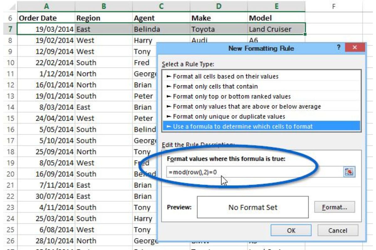
In the “New Formatting Rule” dialog box, select the option that says “Use a formula to determine which cells to format.”
In the formula input box below, enter the formula that will determine which rows to format. For example, if your range starts from cell A1, you can use the formula “=MOD(ROW(),2)=0” to format every other row.
Customize the formatting options such as font color, fill color, or any other desired formatting style for the alternate rows.
Click “OK” to apply the conditional formatting rule to the selected range.

Once the conditional formatting is applied, the specified formatting style will be applied to the alternate rows in the range. This will create a visually appealing pattern that distinguishes one row from the next, allowing for easier reading and analysis of the data.

This technique is particularly useful when working with large tables or datasets, as it helps break up the information and improves readability. By applying conditional formatting to alternate rows, you can enhance the visual structure of your Excel spreadsheets, making it easier to track data and draw attention to important details.

Using Formulas to Shade Alternate Rows

Using formulas to shade alternate rows in Excel is an effective way to quickly apply conditional formatting and create a visually appealing pattern. By leveraging formulas, you can dynamically determine which rows to format based on specific conditions or criteria. Here’s how you can use formulas to shade alternate rows:

Select the range of cells where you want to apply the conditional formatting or ensure that it is already selected. This range should include all the rows you want to format.
Open the Conditional Formatting window by going to the “Home” tab, clicking on the “Conditional Formatting” button, and selecting “New Rule” from the dropdown menu.
In the “New Formatting Rule” dialog box, select the option that says “Use a formula to determine which cells to format.”
In the formula input box below, enter the formula that will define the condition to determine which rows to shade. For example, you can use the formula “=MOD(ROW(),2)=0” to shade every other row.
Customize the formatting options such as font color, fill color, or any other desired formatting style for the shaded rows.
Click “OK” to apply the conditional formatting rule to the selected range.

Upon applying conditional formatting with the formula, the corresponding rows that meet the specified condition will be shaded. The formula evaluates the row number using the MOD function and determines if it is an even or odd row. This approach allows you to dynamically shade alternate rows regardless of changes in the data or the addition/removal of rows.

Using formulas to shade alternate rows not only enhances the visual aesthetics of your Excel spreadsheets but also improves readability and makes it easier to follow and analyze data. This technique is particularly handy when working with large datasets and tables, providing a clear visual distinction between rows and facilitating data interpretation.

Tips for Using Conditional Formatting with Alternate Rows

When using conditional formatting with alternate rows in Excel, there are some tips and considerations that can help you make the most out of this technique. By keeping these tips in mind, you can effectively apply and manage conditional formatting to create visually appealing and easy-to-read spreadsheets. Here are some tips for using conditional formatting with alternate rows:

Choose contrasting colors: Select colors for alternate rows that provide a clear contrast, making it easier to distinguish one row from another. This ensures that the formatting is visually effective and doesn’t cause confusion.
Keep it consistent: Apply the same formatting style to all alternate rows to maintain a consistent and organized appearance. This helps in maintaining readability and a professional look across the spreadsheet.
Consider the overall design: Take into account the overall design and theme of your spreadsheet. Ensure that the alternate row formatting aligns with other formatting elements such as headers, borders, and cell styles to create a cohesive visual presentation.
Combine with other conditional formatting rules: Experiment with combining alternate row formatting with other conditional formatting rules to draw attention to specific data points or highlight significant trends. Used in combination, these rules can provide a comprehensive visual representation of the data.
Use relative references: When writing formulas to shade alternate rows, use relative references instead of absolute cell references. This allows the conditional formatting to adjust automatically if you copy and paste or apply it to other ranges within the spreadsheet.
Test and preview: Preview the conditional formatting before finalizing it to ensure that it achieves the desired effect. Test the formatting with sample data to see how it appears and make any necessary adjustments for optimal results.
Document your rules: If you have complex conditional formatting rules involving multiple formulas or conditions, document them for future reference. This helps in understanding and managing the formatting rules as your spreadsheet evolves.

By following these tips, you can effectively use conditional formatting with alternate rows to improve the visual representation and readability of your Excel spreadsheets. It enables you to present data in a structured and organized manner, making it easier to interpret and analyze information.