Sum Cells That Meet Multiple Criteria With Excel SUMPRODUCT

What is the SUMPRODUCT function in Excel?

The SUMPRODUCT function in Excel is a powerful tool that allows you to sum the product of corresponding values in multiple arrays or ranges. It is particularly useful when you need to perform calculations that involve multiple criteria.

Unlike the traditional SUM function, which can only perform simple addition, the SUMPRODUCT function takes into account the values in multiple arrays or ranges and multiplies them before summing them up. This makes it an invaluable tool for complex calculations.

With the SUMPRODUCT function, you can easily sum the values in a specified range based on specific criteria or conditions. It allows you to perform calculations that would otherwise require multiple nested IF statements or complex array formulas.

The syntax of the SUMPRODUCT function is:

=SUMPRODUCT(array1, array2, ...)

The arrays can be actual ranges of cells, named ranges, or even constants. You can pass multiple arrays as arguments, and the function will multiply the corresponding values in each array and sum them up. If an array contains non-numeric values or empty cells, they will be treated as zeros.

Now that you have an understanding of what the SUMPRODUCT function is, let’s explore how to use it to sum cells that meet multiple criteria in Excel.

Syntax and arguments of the SUMPRODUCT function

The SUMPRODUCT function in Excel has a simple yet flexible syntax. It accepts one or more arrays as arguments and returns the sum of their products.

The basic syntax of the SUMPRODUCT function is:

=SUMPRODUCT(array1, array2, ...)

The arrays can be actual ranges of cells, named ranges, or constants. You can pass multiple arrays as arguments, separated by commas, and the function will multiply the corresponding values in each array and sum them up.

The main argument of the SUMPRODUCT function is the arrays. You can include as few as one array or as many as needed. Each array must have the same dimensions or be of equal length, or else a #VALUE! error will occur.

In addition to arrays, you can also include other arguments within the SUMPRODUCT function:

• Criteria: You can use criteria to filter the values in the arrays before summing them up. This can be done using logical operators such as equals (=), less than (<), greater than (>), or combinations of operators.
• Additional arrays: You can include additional arrays to multiply with the initial arrays. This allows you to perform more complex calculations.

It is important to note that the SUMPRODUCT function treats non-numeric values or empty cells as zeros. Therefore, if an array contains non-numeric values, they will be multiplied as zeros and not affect the final result.

Now that you are familiar with the syntax and arguments of the SUMPRODUCT function, let’s move on to how you can use it to sum cells that meet multiple criteria in Excel.

Using the SUMPRODUCT function to sum cells that meet multiple criteria

The SUMPRODUCT function in Excel is a handy tool when it comes to summing cells that meet multiple criteria. It allows you to specify conditions or criteria and only sum the cells that satisfy those conditions.

To use the SUMPRODUCT function for summing cells with multiple criteria, you need to combine it with other functions such as SUMIF, COUNTIF, and logical operators like equals (=), less than (<), greater than (>), or combinations of operators.

The basic formula to sum cells that meet multiple criteria using the SUMPRODUCT function is:

=SUMPRODUCT((criteria_range1 = criteria1) * (criteria_range2 = criteria2) * range_to_sum)

This formula consists of three parts:

• Criteria: Specify the criteria or conditions that the cells must meet. This can be done by comparing the criteria ranges with the desired criteria values using the equals (=) operator.
• Cell Ranges: Select the cell ranges that you want to sum based on the criteria. This is the range of cells that the SUMPRODUCT function will sum up.

The SUMPRODUCT function multiplies each criteria condition together, resulting in an array of 1s and 0s. The 1s represent the cells that meet all the specified criteria, and the 0s represent the cells that do not meet the criteria.

Finally, the SUMPRODUCT function sums up the values in the range_to_sum based on the corresponding 1s and 0s in the criteria array. It ignores the 0s and adds the values of the cells that meet all the criteria.

With this approach, you can easily sum cells that meet multiple criteria without resorting to complicated nested IF statements or array formulas.

Now, armed with the knowledge of using the SUMPRODUCT function for multiple criteria, let’s dive into a step-by-step guide on how to sum cells with multiple criteria in Excel.

Step-by-step guide to summing cells with multiple criteria using SUMPRODUCT

If you need to sum cells that meet multiple criteria in Excel, the SUMPRODUCT function can come in handy. This step-by-step guide will walk you through the process:

1. Identify the range of cells that you want to sum based on specific criteria. This could be a single column or multiple columns.
2. Identify the criteria you want to use for filtering the cells. For example, you might want to sum the values in a specific column based on the criteria in another column.
3. Set up your criteria range. This is the range of cells that contains the criteria you want to use. Ensure that this range aligns with the range you identified in step 1.
4. Decide on the criteria values you want to use. These values will be compared to the criteria range to determine which cells to include in the sum.
5. Construct the SUMPRODUCT formula. Start by entering the equal (=) operator, followed by the SUMPRODUCT function. Inside the function, use parentheses to group the criteria comparisons. Multiply the criteria comparisons together using the asterisk (*) operator. Finally, multiply the resulting array by the range of cells you want to sum.
6. Close the formula with a closing parenthesis and press Enter to calculate the sum.
7. Verify that the sum is accurate and adjust the criteria or range if necessary.

By following these steps, you can easily use the SUMPRODUCT function to sum cells that meet multiple criteria in Excel. This approach saves you time and effort compared to manually filtering and summing cells based on each criterion.

Now that you have a clear understanding of how to use the SUMPRODUCT function for multiple criteria, it’s time to explore some practical examples that demonstrate its capabilities.

Example 1: Summing cells based on multiple criteria in a single column

Let’s say you have a spreadsheet that tracks sales data, and you want to sum the sales total for a specific product in a single column based on multiple criteria, such as the region and month. Here’s how you can use the SUMPRODUCT function to accomplish this:

1. Identify the range of cells that contains the sales data. Let’s assume the sales data is in column B.
2. Identify the criteria ranges for the region and month. For example, the region criteria could be in column A, and the month criteria could be in column C.
3. Enter the desired criteria values in separate cells. For instance, if you want to sum the sales for the “North” region in the “January” month, you would enter “North” in one cell and “January” in another.
4. In a separate cell, construct the SUMPRODUCT formula. Start with the equal (=) operator, followed by SUMPRODUCT. Inside the function, specify the criteria range for the region and compare it to the criteria value using the equals (=) operator. Repeat this step for the month criteria and value. Multiply the two comparisons together. Finally, multiply the resulting array by the range of sales data (column B).
5. Press Enter to calculate the sum of sales that meet the specified criteria.

By following these steps and adjusting the criteria values as needed, you can easily sum the sales total for a specific product based on multiple criteria in a single column. This provides a more efficient and dynamic way to analyze your data.

Now that you’ve seen an example of summing cells based on multiple criteria in a single column, let’s explore another example that demonstrates how to sum cells based on multiple criteria in multiple columns.

Example 2: Summing cells based on multiple criteria in multiple columns

In some cases, you may need to sum cells based on multiple criteria that are spread across multiple columns. Let’s consider a scenario where you have a sales dataset with columns for product, region, and month, and you want to find the total sales for a specific product in a specific region and month. Here’s how you can use the SUMPRODUCT function for this scenario:

1. Identify the range of cells that contains the sales data. Let’s assume the sales data is in column D.
2. Identify the criteria ranges for the product, region, and month. These could be in columns A, B, and C, respectively.
3. Enter the desired criteria values in separate cells for product, region, and month.
4. In a separate cell, construct the SUMPRODUCT formula. Start with the equal (=) operator, followed by SUMPRODUCT. Inside the function, specify the criteria range for the product and compare it to the criteria value using the equals (=) operator. Repeat this step for the region and month criteria and values. Multiply the three comparisons together. Finally, multiply the resulting array by the range of sales data (column D).
5. Press Enter to calculate the sum of sales that meet all the specified criteria.

By following these steps and adjusting the criteria values as needed, you can easily sum the sales for a specific product in a specific region and month, even when the criteria are spread across multiple columns. This allows for more precise analysis and reporting of your sales data.

The flexibility of the SUMPRODUCT function makes it a powerful tool for summing cells based on multiple criteria in multiple columns. With just a few steps, you can obtain accurate results and gain deeper insights into your data.

Now that you have seen an example of summing cells based on multiple criteria in multiple columns, let’s explore an advanced example that demonstrates how to use logical operators (AND and OR) with the SUMPRODUCT function.

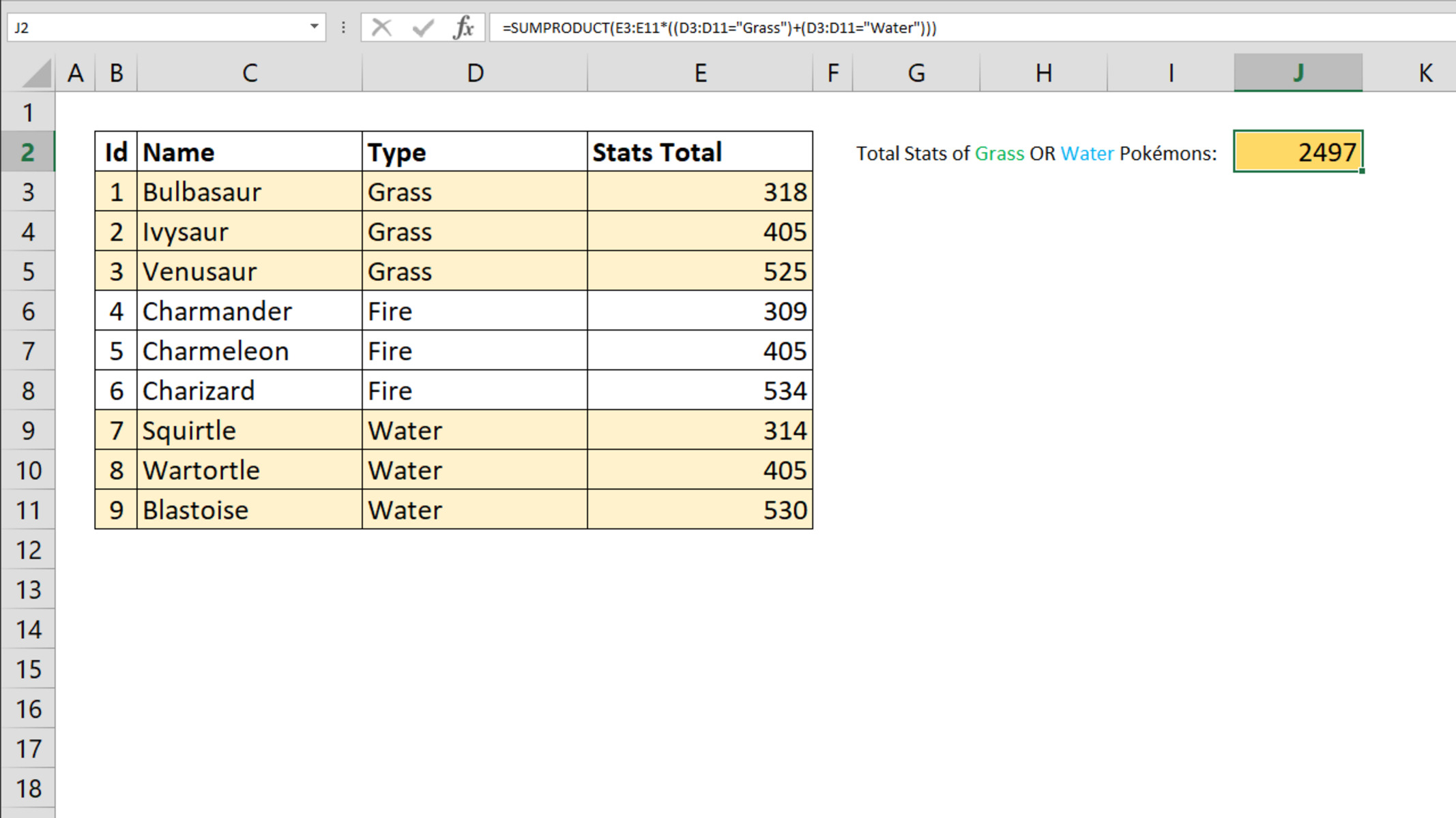
Example 3: Summing cells based on multiple criteria with logical operators (AND and OR)

When summing cells based on multiple criteria, you may need to use logical operators such as AND and OR to create more complex conditions. Let’s consider a situation where you want to sum the sales for a specific product in a specific region for either the “January” or “February” month. Here’s how you can use the SUMPRODUCT function with logical operators:

1. Identify the range of cells that contains the sales data. Let’s assume the sales data is in column E.
2. Identify the criteria ranges for the product, region, and month. These could be in columns A, B, and C, respectively.
3. Enter the desired criteria values in separate cells for product and region. For the month criteria, you can either use a cell that contains “January” or create two separate cells for “January” and “February”.
4. In a separate cell, construct the SUMPRODUCT formula. Start with the equal (=) operator, followed by SUMPRODUCT. Inside the function, specify the criteria range for the product and compare it to the criteria value. Use the equals (=) operator for the product and region criteria. For the month criteria, use the OR operator to check if it matches either “January” or “February”. Multiply the three comparisons together. Finally, multiply the resulting array by the range of sales data (column E).
5. Press Enter to calculate the sum of sales that meet the specified criteria.

By following these steps and adjusting the criteria values as needed, you can easily sum the sales for a specific product in a specific region for multiple months, using logical operators to create more dynamic conditions. This enables you to perform complex analysis and gain insights from your data.

The SUMPRODUCT function combined with logical operators gives you the flexibility to create sophisticated criteria for summing cells based on multiple conditions. With just a few adjustments, you can tackle more complex scenarios and extract meaningful information from your data.

Now that you have learned how to use logical operators with the SUMPRODUCT function, let’s move on to some tips and tricks to effectively utilize this powerful Excel function.

Tips and tricks for using the SUMPRODUCT function effectively

The SUMPRODUCT function is a versatile tool in Excel that allows you to sum cells based on multiple criteria. Here are some tips and tricks to optimize your usage of the SUMPRODUCT function:

• 1. Understand array multiplication: The key to the SUMPRODUCT function is the multiplication of arrays. Make sure you understand how arrays work in Excel and how they interact with each other.
• 2. Handle non-numeric values: The SUMPRODUCT function treats non-numeric values as zeros. If your criteria range contains non-numeric values, consider using the IF or ISNUMBER functions to handle them appropriately.
• 3. Use wildcard characters: You can combine the SUMPRODUCT function with wildcard characters, such as asterisks (*) or question marks (?), to match patterns or partial values in your criteria.
• 4. Utilize logical operators: Take advantage of logical operators like AND, OR, and NOT to create more complex conditions for your criteria. This allows for greater flexibility in defining the cells to include in the sum.
• 5. Use named ranges: Named ranges can make your formulas more readable and organized. Consider assigning names to your criteria ranges and range to sum to make your SUMPRODUCT formula easier to understand.
• 6. Combine with other functions: The SUMPRODUCT function can be combined with other Excel functions like SUMIF, COUNTIF, and AVERAGEIF to perform more complex calculations. Explore different possibilities to enhance your data analysis.
• 7. Use cell references: Instead of hardcoding your criteria values directly in the formula, use cell references. This allows you to easily change the criteria without modifying the formula itself.
• 8. Test and validate: After setting up your SUMPRODUCT formula, test it with different scenarios and validate the results to ensure accuracy. Double-check your criteria and ranges to avoid errors.

These tips and tricks will help you effectively utilize the SUMPRODUCT function to sum cells based on multiple criteria in Excel. Remember to experiment and explore its capabilities to make the most of your data analysis tasks.

Now that you have a solid understanding of the SUMPRODUCT function and how to use it effectively, you can confidently tackle complex calculations and gain valuable insights from your data.