
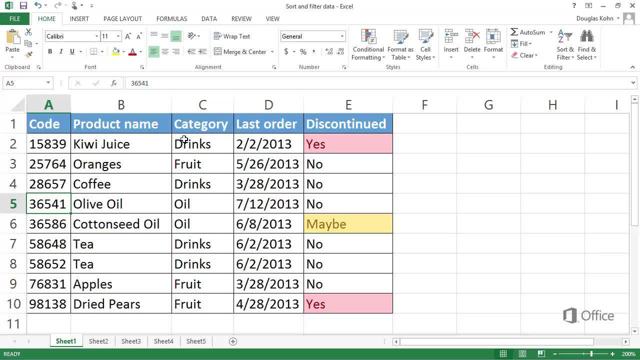
What is a table in Excel?
A table in Excel is a powerful feature that allows users to organize and analyze related data efficiently. It provides a structured layout with built-in functionality for sorting, filtering, and analyzing data. Unlike a regular range of cells, a table has distinct characteristics that make it an excellent tool for managing and manipulating data.
Creating a table in Excel is simple. You can either convert an existing range of data into a table or start from scratch by entering your data directly into the table. To convert a range into a table, select the range, go to the “Insert” tab, and click on the “Table” button. Excel will automatically detect the range and convert it into a table with predefined column names.
When you create a table, Excel applies various formatting options, such as alternating row colors and banded columns, to enhance the visual appeal and readability of the data. In addition, it assigns a table name to facilitate easy referencing and includes filter buttons in the table header, allowing you to quickly filter data based on specific criteria.
One of the significant advantages of using tables in Excel is that they provide dynamic functionality. As you add or remove data to the table, the table automatically expands or contracts, maintaining the integrity of the table structure. This feature is beneficial when dealing with ever-changing data sets where you need to update or analyze information frequently.
With tables, you can also take advantage of Excel’s powerful sorting capabilities. Sorting data in a table allows you to arrange it in a specific order based on one or more columns. This functionality is particularly useful when you have large amounts of data and need to find specific information quickly.
In the next section, we will explore how to sort data in a table in Excel, including sorting by a single column, multiple columns, and applying custom sorting techniques.
Creating a table in Excel
Creating a table in Excel is a straightforward process that enables you to organize and analyze your data more effectively. There are two common methods to create a table in Excel: converting an existing range of data into a table or starting from scratch by entering your data directly into the table.
To convert an existing range into a table, first, select the range of cells that you want to convert. This range could include headers for each column, but it’s not mandatory. Once the range is selected, go to the “Insert” tab in the Excel ribbon and click on the “Table” button. Excel will automatically detect the range you selected and display the “Create Table” dialog box.
In the “Create Table” dialog box, you can customize various table options such as the table style, table name, and whether or not your data has headers. It’s recommended to have headers in your table as they provide clear labels for each column and make it easier to work with and analyze the data. After confirming the options, click on the “OK” button, and Excel will instantly convert your selected range into a table.
If you prefer to start with a new table and enter your data directly, navigate to a blank worksheet in Excel. Enter your data starting from the top left cell, making sure to include column headers for each column. Once you have entered the data, select the range, go to the “Insert” tab, and click on the “Table” button. Again, the “Create Table” dialog box will appear, allowing you to define the table options before confirming and creating the table.
When you create a table in Excel, it not only visually enhances the appearance of your data with predefined formatting but also provides several useful features. The table is given a unique name, which can be referenced in formulas and functions. Excel also adds filter buttons to the header row, enabling you to quickly filter and sort your data based on specific criteria. Additionally, tables in Excel are dynamic, meaning that when you add or remove data from the table, the table expands or contracts automatically to accommodate the changes.
Creating a table in Excel is a powerful way to organize and manipulate your data. Whether you convert an existing range or start from scratch, tables provide a structured and dynamic framework that streamlines your data analysis tasks.
Benefits of using tables for related data
Tables are an invaluable tool in Excel for managing and analyzing related data. They offer several benefits that make them essential for organizing and working with large datasets in a structured and efficient manner.
One of the key advantages of using tables is their ability to maintain data integrity. When you create a table in Excel, it automatically assigns unique column names to each field. This ensures that your data remains consistent and easily identifiable, even as you add or remove rows or columns. Additionally, tables allow you to input data validation rules, preventing the entry of incorrect or invalid values. This helps in maintaining data accuracy and reducing potential errors.
Tables also provide a visual distinction for your data. When you convert a range of cells into a table, Excel automatically applies a stylish format to the table, with alternating row colors and banded columns. This makes it easier to read and analyze the data at a glance. Furthermore, tables are equipped with filter buttons in the header row, enabling you to quickly filter and narrow down the data based on specific criteria. This feature is especially useful when dealing with large datasets where finding specific information can be time-consuming.
Another advantage of using tables is their dynamic nature. As you add or remove data to the table, the table automatically adjusts its size and formatting to accommodate the changes. This eliminates the need for manually adjusting cell references or range names, saving you time and effort. Moreover, tables allow you to use structured references in formulas instead of traditional cell references. This makes formulas more readable and less prone to errors, as you can easily refer to specific columns or calculations within the table.
Excel tables also integrate well with other Excel features, such as PivotTables and charts. You can easily convert a table into a PivotTable for more advanced data analysis and reporting, or create dynamic charts that update automatically as the table data changes. Tables enhance the overall functionality and versatility of Excel, allowing you to extract meaningful insights from your data with ease.
Working with related data becomes much more efficient and convenient when using Excel tables. Their data integrity, visual distinction, dynamic nature, and seamless integration with other Excel features make tables a powerful tool for organizing, analyzing, and presenting your data in a structured manner.
Sorting data in a table
Sorting data in a table is a fundamental feature of Excel that allows you to arrange your data in a specific order based on one or more columns. Sorting is particularly useful when working with large datasets, as it enables you to easily locate and analyze information within the table.
In Excel, you can sort data in a table in ascending or descending order. Ascending order means that the data will be arranged from the smallest value to the largest value, while descending order will arrange the data in the opposite direction, from the largest value to the smallest value. Sorting can be done on a single column or multiple columns, providing flexibility in organizing your data.
To sort data in a table, first select any cell within the table. Then, navigate to the “Data” tab in the Excel ribbon and click on the “Sort” button. Excel will prompt you to choose the column or columns you want to use for sorting. You can select one or multiple columns by specifying the criteria for each column.
When sorting data in a table, Excel provides several options to enhance the sorting process. You can sort data with a custom sort, which allows you to define a specific order for sorting. For example, you can sort a list of months in a non-chronological order by specifying a custom sort order. Additionally, you can sort data with a formula, where Excel uses a formula to determine the sorting order based on specific criteria.
Excel also allows you to sort data with a custom list. This feature is helpful when you have a specific list of values that you want to sort by. For example, you can create a custom list for sorting data by priority or alphabetically based on a specific sequence of values.
Furthermore, you can sort data in a table based on icons or color. If you have applied conditional formatting to your data with icons or color scales, you can sort the data based on the visual cues. This can be useful when you want to prioritize or analyze specific data points within the table.
It is important to note that when sorting data in a table, Excel automatically expands the selection to include all columns in the table. This ensures that the data remains intact and that associated values in other columns are not disconnected from their corresponding data.
Overall, sorting data in a table is a powerful feature in Excel that allows you to organize and analyze your data efficiently. Whether you need to sort by a single column, multiple columns, apply custom sorting, or utilize advanced sorting options, Excel provides the tools to help you manipulate and arrange your data in a way that best suits your needs.
Sorting data by a single column
Sorting data by a single column in Excel is a straightforward process that allows you to rearrange the rows of your table in a specific order based on the values in that column. Sorting by a single column is useful when you want to organize your data in ascending or descending order to identify trends or easily locate specific data points.
To sort data by a single column in Excel, start by selecting any cell within the table. Then, navigate to the “Data” tab in the Excel ribbon and click on the “Sort” button. Excel will prompt you to select the column you want to use for sorting. Choose the desired column, and specify whether to sort in ascending or descending order.
When you sort data by a single column, Excel rearranges the entire table based on the values in that column. For example, if you have a table of sales data with a “Sales Amount” column, sorting in ascending order will arrange the rows from the lowest sales amount to the highest, while sorting in descending order will arrange the rows from the highest to the lowest sales amount.
Excel also provides additional options when sorting by a single column. For example, you can choose to sort by cell color or font color. This is useful when you have applied conditional formatting to your data and want to prioritize or analyze specific data points based on their visual cues.
Additionally, you can sort by the number or text length in a column. Sorting by number will arrange the rows based on the numerical values in the selected column, while sorting by text length will arrange the rows based on the length of the text in the column.
Another option when sorting by a single column is to sort by cell icon. If you have applied icon sets to your data, Excel allows you to sort the data based on the icons assigned to each value in the column.
Excel tables also provide the ability to sort by a specific order. This feature is useful when you want to define a custom sort order for your data. You can create a custom list of values and specify the desired order for sorting.
Sorting data by a single column in Excel is a powerful tool for organizing and analyzing your data. By rearranging the rows based on the values in a specific column, you can identify patterns, trends, and outliers, making it easier to extract relevant insights from your data.
Sorting data by multiple columns
In Excel, you can sort data by multiple columns to further refine the order in which your data is arranged. Sorting by multiple columns allows you to prioritize and organize your data based on multiple criteria, helping you to gain deeper insights and uncover patterns within your dataset.
To sort data by multiple columns in Excel, start by selecting any cell within the table. Then, navigate to the “Data” tab in the Excel ribbon and click on the “Sort” button. In the Sort dialog box, you can specify the primary column to sort by from the ‘Sort by’ dropdown menu. Next, click on the ‘Add Level’ button to define additional sorting levels. You can add up to 64 sorting levels in Excel.
When you sort by multiple columns, Excel applies the sorting criteria in the order they are specified. The first column selected becomes the primary sorting level, followed by the second column, and so on. This means that if there are any duplicate values in the first column, Excel will sort them based on the values in the second column. The sorting process continues in this manner until all specified columns have been considered.
Sorting by multiple columns allows you to have a more granular control over the order of your data. For example, you can sort a table of sales data by the ‘Region’ column as the primary sorting level, and then by the ‘Sales Amount’ column as the secondary level. This will arrange the data first by region, and within each region, sort by the sales amount in ascending or descending order.
Within the Sort dialog box, you can also customize the sorting order for each column. By default, Excel sorts in ascending order, but you can change it to descending order as needed. Furthermore, you have the option to sort numbers as text or dates as text if you prefer to arrange them in alphabetical order instead of their numerical or chronological order.
Sorting by multiple columns is particularly useful when you have complex datasets with multiple factors influencing the order of the data. By sorting on multiple criteria, you can accurately prioritize and analyze your data. This feature helps you uncover relationships, identify trends, and gain a deeper understanding of your data.
Excel provides a robust set of tools to sort data by multiple columns, giving you the flexibility to arrange your information in a specific order that best suits your needs. Whether you are analyzing sales data, customer information, or any other type of dataset, sorting by multiple columns can provide valuable insights into your data.
Sorting data in ascending order
Sorting data in ascending order is a common operation in Excel that allows you to arrange your data from the smallest value to the largest value. Sorting in ascending order is useful when you want to identify trends, rank data, or analyze it in a specific order.
To sort data in ascending order in Excel, start by selecting any cell within the table. Then, navigate to the “Data” tab in the Excel ribbon and click on the “Sort” button. In the Sort dialog box, choose the column you want to sort by from the ‘Sort by’ dropdown menu. By default, Excel sorts in ascending order, so there is no need to make any further changes.
When you sort data in ascending order, Excel rearranges the rows of your table based on the values in the selected column. For numerical values, the smallest value will be at the top, and the largest value will be at the bottom. For text values, the sorting is done alphabetically, with the A’s appearing before the B’s, and so on.
Sorting data in ascending order can be applied to single or multiple columns in your table. You can sort by a single column when you want to organize your data based on a specific factor, such as sales amount or employee names. When sorting by multiple columns, Excel applies the ascending order to each column in the order they were specified. This allows you to sort on multiple criteria, giving you more control over the arrangement of your data.
In addition to sorting entire columns, you can also sort a specific range of data within your table. This is useful when you only want to sort a portion of your data, rather than the entire dataset. By selecting the desired range before applying the sort, you can sort specific rows or columns within your table.
Excel provides a range of additional options to customize the ascending order sorting process. For example, you can sort by cell color or font color, which is particularly useful when you have applied conditional formatting to your data. You can also sort by the number or text length within a column, where Excel arranges the rows based on the numerical value or the length of the text in the column.
Sorting data in ascending order is a valuable feature in Excel that allows you to organize your data. Whether you are working with numerical or text data, sorting in ascending order helps you identify patterns, rank data, and analyze it in a specific order that best suits your needs.
Sorting data in descending order
Sorting data in descending order is a useful feature in Excel that allows you to arrange your data from the largest value to the smallest value. Sorting in descending order is beneficial when you want to identify high-ranking or top-performing data points, analyze data in a reverse order, or find the largest values within your dataset.
To sort data in descending order in Excel, begin by selecting any cell within the table. Then, navigate to the “Data” tab in the Excel ribbon and click on the “Sort” button. In the Sort dialog box, choose the column you want to sort by from the ‘Sort by’ dropdown menu. By default, Excel sorts in ascending order, so you need to change the order to descending by selecting ‘Descending’ in the ‘Order’ dropdown menu.
When you sort data in descending order, Excel reorganizes the rows of your table based on the values in the selected column. Numerical values will be arranged from the largest to the smallest, while text values will be sorted in reverse alphabetical order, starting from Z and proceeding to A.
Similar to sorting in ascending order, sorting data in descending order can be applied to single or multiple columns in your table. By specifying additional sorting levels, you can create more complex sorting scenarios where Excel first sorts based on the primary factor, and within each group, arranges the data in descending order based on the secondary factor.
Excel also provides several options to further customize the descending order sorting process. For example, you can sort by cell color or font color, allowing you to prioritize or identify specific data points based on their visual cues. Sorting by the number or text length in a column enables you to arrange the rows based on the numerical value or the length of the text, from the longest to the shortest.
In addition to sorting entire columns, you can also sort a specific range of data within your table. This is useful if you only want to sort a portion of your data, rather than the entire dataset. By selecting the desired range before applying the sort, you can sort specific rows or columns within your table.
Sorting data in descending order is a powerful feature in Excel that allows you to analyze and rank your data in reverse order. Whether you are working with numerical or text data, sorting in descending order helps you identify top performers, analyze data from the largest to the smallest values, and uncover important insights within your dataset.
Sorting data with custom sort
Excel provides the ability to sort data with a custom sort, allowing you to define a specific order for sorting your data. Custom sorting is particularly useful when you want to arrange your data based on a specific sequence or prioritize certain values over others.
To sort data with a custom sort in Excel, start by selecting any cell within the table. Then, navigate to the “Data” tab in the Excel ribbon and click on the “Sort” button. In the Sort dialog box, choose the column you want to sort by from the ‘Sort by’ dropdown menu. Next, click on the ‘Options’ button to access additional sorting options.
Within the ‘Options’ dialog box, select the ‘Custom Lists’ tab. Here, you can view and manage the custom lists that are available in Excel. A custom list is a user-defined sequence of values that can be used for custom sorting. Excel provides some built-in custom lists, such as days of the week and months of the year, but you can also create your own custom lists.
To create a custom list, click on the ‘Import’ button and follow the prompts to select a range of cells containing the values you want to use for sorting. Once the custom list is imported, you can use it for sorting by selecting it in the ‘Order’ dropdown menu within the ‘Sort’ dialog box.
Sorting data with a custom sort gives you control over the order in which your data appears. For example, if you have a column with priority values ranging from low to high, you can create a custom list to sort the data in a specific order that aligns with your priority levels.
Custom sorting is not limited to a single column; you can apply it to multiple columns in your table. This means you can have distinct custom sort sequences for different columns, allowing you to achieve more granular control over the sorting order of your data.
When using custom sorting, it’s important to note that Excel retains the custom sort order even if you add or remove data from the table. This ensures that the specified order remains consistent, making it easier to keep track of specific values and maintain the integrity of your data.
Sorting data with a custom sort provides a flexible and powerful tool for arranging your data in a customized way. By defining a specific order or priority level for sorting, you can prioritize certain values, categorize data based on specific sequences, and tailor the sorting process to your unique data requirements.
Sorting data with a specific order
In Excel, you have the ability to sort data with a specific order, allowing you to sort your data in a predetermined sequence that aligns with your specific requirements. Sorting data with a specific order is useful when you want to prioritize certain values, arrange data in a non-traditional or custom order, or categorize data based on a specific sequence.
To sort data with a specific order in Excel, start by selecting any cell within the table. Then, navigate to the “Data” tab in the Excel ribbon and click on the “Sort” button. In the Sort dialog box, choose the column you want to sort by from the ‘Sort by’ dropdown menu. Next, click on the ‘Options’ button to access additional sorting options.
Within the ‘Options’ dialog box, select the ‘Order’ dropdown menu. By default, Excel sorts data in ascending or descending order. However, you can select the ‘Custom List’ option from the dropdown menu to specify a specific order for sorting.
To define a specific order, you can either choose from Excel’s built-in custom lists, such as days of the week or months of the year, or create your own custom list. To create a custom list, click on the ‘Import’ button and follow the prompts to select a range of cells containing the values you want to use for sorting in the specific order.
Once you’ve selected or created the specific order, Excel will sort the data according to that order. This allows you to arrange the data in a manner that aligns with your unique requirements, regardless of the typical alphabetical or numerical sorting.
Sorting data with a specific order is not limited to a single column; you can apply it to multiple columns within your table. Each column can have its own specific order, giving you the flexibility to customize the sorting sequence for different data categories.
It’s important to note that when using a specific order, Excel retains the defined order even if you add or remove data from the table. This ensures that the intended order remains intact, allowing you to maintain consistency and easily identify and categorize specific values within your dataset.
Sorting data with a specific order provides a powerful feature in Excel that allows for customized and tailored sorting sequences. By applying a specific order to your data, you can prioritize values, categorize data based on a unique sequence, and arrange your data in a meaningful and personalized way.
Sorting data with a formula
In Excel, you can sort data with a formula, which allows you to define specific criteria for sorting your data. Sorting data with a formula is useful when you want to arrange your data based on complex conditions, custom calculations, or specific requirements that cannot be achieved through traditional sorting methods.
To sort data with a formula in Excel, start by selecting any cell within the table. Then, navigate to the “Data” tab in the Excel ribbon and click on the “Sort” button. In the Sort dialog box, choose the column you want to sort by from the ‘Sort by’ dropdown menu.
In the ‘Options’ section of the Sort dialog box, select the ‘Sort on’ dropdown menu and choose ‘Values’ or ‘Cell Color’. If you choose ‘Values’, you can then specify the custom formula you want to use for sorting. The formula can be created using a combination of functions, logical operators, and cell references.
For example, suppose you have a table of sales data with columns for ‘Product’, ‘Quantity’, and ‘Price’. You can use a formula to sort the data based on the total sale amount, calculated by multiplying the ‘Quantity’ and ‘Price’ columns for each row.
=Quantity * Price
By including this formula in the sorting criteria, Excel will arrange the data based on the calculated total sale amount, sorting in ascending or descending order as specified.
Sorting data with a formula provides great flexibility, as you can use any combination of functions, conditions, and calculations to define the sorting order. This enables you to create complex sorting rules based on your unique requirements and allows for sorting based on multiple columns or even across different worksheets or workbooks.
It’s important to note that when sorting data with a formula, Excel dynamically recalculates the values based on the formula each time the sort is performed. This ensures that the sorting order is always up to date, reflecting any changes in the source data or the formula itself.
Sorting data with a formula provides a powerful tool for arranging and analyzing data in Excel. By applying custom calculations and logical rules, you can sort your data based on specific criteria and achieve a more targeted and meaningful data arrangement for your analysis and reporting needs.
Sorting data with a custom list
In Excel, you can sort data with a custom list, allowing you to define a specific order for sorting your data based on a customized sequence of values. Sorting data with a custom list is useful when you want to arrange your data according to non-alphabetical or non-numerical criteria, or when you have a specific order in mind that is not based on traditional sorting methods.
To sort data with a custom list in Excel, start by selecting any cell within the table. Then, navigate to the “Data” tab in the Excel ribbon and click on the “Sort” button. In the Sort dialog box, choose the column you want to sort by from the ‘Sort by’ dropdown menu.
In the ‘Options’ section of the Sort dialog box, select the ‘Sort on’ dropdown menu and choose ‘Values’. Then, select the ‘Order’ dropdown menu, and choose the ‘Custom Lists’ option.
Excel provides some built-in custom lists, such as days of the week or months of the year. If your desired custom order aligns with one of these built-in lists, you can select it directly from the ‘Order’ dropdown menu.
If your custom order is not included in the built-in lists, you can create your own custom list in Excel. To do this, click on the ‘Import’ button within the ‘Custom Lists’ tab of the ‘Sort’ dialog box. Then, select a range of cells that contains the values in the order you want for sorting. Once imported, Excel will use your custom list to sort the data accordingly.
Sorting data with a custom list allows for flexibility and customization in sorting your data. You can create custom lists for various purposes, such as priority levels, educational grades, or specific categorizations. By using this feature, you can sort your data in a way that suits your specific needs and preferences.
It’s important to note that when using a custom list, Excel retains the defined order even if you add or remove data from the table. This ensures that the intended order remains intact and consistent, making it easier to identify and categorize specific values within your dataset.
Sorting data with a custom list provides a powerful tool for arranging your data in a personalized and meaningful way. By defining a specific order for your data, you can align the data with your own custom criteria or categorization, making the sorting process more tailored to your unique requirements.
Sorting data with icons or color
In Excel, you can sort data with icons or color, allowing you to arrange your data based on visual cues and highlighting specific values or categories. Sorting data with icons or color is useful when you have applied conditional formatting to your data and want to prioritize, categorize, or analyze your data based on the visual representations.
To sort data with icons or color in Excel, start by selecting any cell within the table. Then, navigate to the “Data” tab in the Excel ribbon and click on the “Sort” button. In the Sort dialog box, choose the column you want to sort by from the ‘Sort by’ dropdown menu.
In the ‘Options’ section of the Sort dialog box, select the ‘Sort on’ dropdown menu and choose either ‘Cell Icon’ or ‘Cell Color’, depending on the visual cue you want to use for sorting.
If you have applied icon sets to your data using conditional formatting, selecting the ‘Cell Icon’ option will allow you to sort the data based on the icons assigned to each value in the selected column. For example, if you have a column with traffic light icons indicating performance levels, you can sort the data to prioritize the highest or lowest performance levels.
If you have applied cell color formatting to your data, selecting the ‘Cell Color’ option will enable you to sort the data based on the color assigned to each value. This is useful when you want to categorize or prioritize data based on specific color codes.
Sorting data with icons or color provides a visual method for analyzing your data. By sorting based on the icons or color, you can quickly identify trends, prioritize values, or group data based on common characteristics.
It’s important to note that when sorting data with icons or color, Excel considers the visual cues rather than the underlying values. This means that the sorting is done based on the assigned icons or color, not the actual values in the column.
Sorting data with icons or color is not limited to a single column; you can apply it to multiple columns within your table. This allows you to sort and analyze data based on different visual cues and highlight specific patterns or trends across multiple criteria.
Sorting data with icons or color is a powerful feature in Excel, leveraging visual representations to enhance data analysis. By sorting based on the icons or color, you can quickly identify and analyze data based on specific characteristics, giving you a more intuitive way to interpret and prioritize your data.
Undoing a sort
In Excel, if you accidentally sort your data or want to revert back to the original order, you can easily undo the sort operation. Undoing a sort allows you to restore the original arrangement of your data and undo any unintended changes made during the sorting process.
To undo a sort in Excel, you can use the Undo button or the keyboard shortcut. The Undo button is located in the Quick Access Toolbar at the top left of the Excel window. Simply click on the Undo button, represented by an arrow pointing to the left, or use the keyboard shortcut Ctrl + Z.
By clicking the Undo button or pressing the Ctrl + Z shortcut, Excel will revert the sorting operation and restore the data to its previous unsorted state. This applies to the most recent sort operation that was performed in the worksheet.
It’s important to note that undoing a sort not only brings back the original order of the data but also undoes any changes made to the associated rows or columns. This means that any changes made to other cells or data within the sorted range will also be undone.
If you want to undo multiple sort operations or undo a sort that was performed a while ago, you can use the Undo History feature in Excel. This feature allows you to access a list of recent actions and select the specific sort operation you want to undo.
In addition to undoing a sort, Excel also provides the Redo button or the keyboard shortcut Ctrl + Y, which allows you to redo a previously undone sort operation. This can be useful if you accidentally undo a sort or change your mind about reverting the sort.
Undoing a sort is a handy feature in Excel that allows you to quickly and easily revert back to the original order of your data. It provides a safety net when sorting data, ensuring that any unintended sorting changes can be easily corrected without affecting the integrity of your data.
Sorting data with headers
In Excel, sorting data with headers is a convenient feature that allows you to include or exclude the header row when sorting your data. Sorting data with headers ensures that the column labels or headers remain aligned with their respective data during the sorting process.
By default, when you sort data in Excel, the header row is included in the sorting range. This means that the header row is treated as data and rearranged according to the values in the selected column. This can be useful when you want to sort the entire table, including the header row.
However, in some cases, you may prefer to exclude the header row from the sorting operation to keep the header row intact at the top of your table. This is particularly useful when you have complex headers or want to preserve the order of your column labels while sorting the data.
To sort data with headers in Excel, start by selecting any cell within the table. Then, navigate to the “Data” tab in the Excel ribbon and click on the “Sort” button. In the Sort dialog box, choose the column you want to sort by from the ‘Sort by’ dropdown menu.
In the ‘Options’ section of the Sort dialog box, you can check or uncheck the ‘My data has headers’ box to include or exclude the header row from the sorting operation.
If the ‘My data has headers’ box is checked, Excel will treat the header row as part of the sorting range. In this case, the header row will be rearranged with the rest of the data based on the selected column.
If the ‘My data has headers’ box is unchecked, Excel will not include the header row in the sorting range. The header row will remain in place at the top of your table while only the data below the header row will be rearranged.
Sorting data with headers provides flexibility in managing your data without compromising the integrity of your table. Whether you want to include or exclude the header row during sorting, Excel gives you the option to align the data and headers according to your specific requirements.
It’s worth noting that when sorting data with headers, Excel automatically expands the selection to include all columns in the table. This ensures that the data remains intact and that associated values across different columns are not disconnected from their corresponding data.
Sorting data with headers is a valuable feature in Excel that helps maintain the structure and organization of your table, especially when working with large datasets. It allows for a seamless sorting experience while preserving the alignment of headers and their associated data in a logical and visually organized manner.
Sorting data without headers
In Excel, you have the option to sort data without headers, which allows you to arrange your data based on its values alone, without considering the header row. Sorting data without headers can be useful when you have a range of data without clear column labels or when you want to focus solely on the data values themselves.
To sort data without headers in Excel, start by selecting any cell within the range of data you want to sort. Then, navigate to the “Data” tab in the Excel ribbon and click on the “Sort” button. In the Sort dialog box, choose the column you want to sort by from the ‘Sort by’ dropdown menu.
In the ‘Options’ section of the Sort dialog box, you can uncheck the ‘My data has headers’ box to indicate that your data does not include a header row.
When you sort data without headers, Excel assumes that the first row in the selected range is part of the data, and it treats it as such during the sorting operation. Excel will rearrange the rows based on the values in the selected column, without considering any row as a header.
It’s important to note that when sorting data without headers, Excel does not automatically add header labels to the sorted results. The first row of the selected range will still appear as data after sorting. If you want to manually add headers to the sorted data, you can do so by inserting a new row at the top of the sorted range and entering the appropriate column labels.
Sorting data without headers can be particularly useful when working with data from external sources or when analyzing data where the first row does not represent clear column labels. This allows you to focus on the data values themselves without interference from potentially misleading or irrelevant header labels.
When sorting data without headers, it’s worth considering the potential impact on data analysis or further processing. Without clear column labels, it may be more challenging to interpret the sorted results or perform calculations alongside the data. Therefore, it’s important to ensure that the absence of headers does not hinder subsequent data analysis or understanding.
Sorting data without headers provides flexibility in managing and analyzing your data in Excel. By focusing solely on the values within the data range, you can arrange the data based purely on its numeric or textual properties, enabling a more direct analysis or exploration of the dataset.
Sorting data in a specific range
In Excel, you have the ability to sort data in a specific range, allowing you to sort a subset of data within your worksheet rather than the entire dataset. Sorting data in a specific range is useful when you want to focus on a particular section of data or when you want to maintain the order of other unrelated data in your worksheet.
To sort data in a specific range in Excel, start by selecting the range of cells you want to sort. This can be a single column or a range of columns, and it can include any number of rows. Once the range is selected, navigate to the “Data” tab in the Excel ribbon and click on the “Sort” button. In the Sort dialog box, choose the column you want to sort by from the ‘Sort by’ dropdown menu.
By default, Excel uses the entire column as the sorting range. However, if you have a specific range selected, Excel will automatically detect and sort only within that selected range instead of the entire column.
Sorting data in a specific range allows you to sort a subset of data independently, preserving the arrangement of other data in your worksheet. For example, if you have a worksheet with multiple tables or unrelated data, you can sort each table or specific range individually without affecting the order of other tables or ranges.
When sorting data in a specific range, it’s important to consider that Excel may still adjust the selection to include any associated columns adjacent to the sort range. This ensures that the data remains intact, and associated values from other columns are not disconnected from their corresponding data during the sorting process.
Sorting data in a specific range provides flexibility and control over your sorting operations, allowing you to focus on and arrange only the desired subset of data. This feature is particularly helpful in complex worksheets with multiple tables or when you want to maintain the order of other unrelated data while sorting a specific range within the worksheet.
It’s worth noting that when sorting data in a specific range, Excel does not automatically apply the sorting order to the unselected data. If you want to sort the entire column or multiple columns, you will need to select the appropriate range explicitly.
Sorting data in a specific range empowers you to organize and analyze data selectively, saving time and effort while maintaining the integrity and structure of your overall worksheet.
Sorting data in a filtered table
In Excel, you can sort data in a filtered table, which allows you to apply sorting operations to a subset of data that is currently filtered based on specific criteria. Sorting data in a filtered table enables you to further refine and analyze your data, taking into account only the visible records that meet the applied filters.
To sort data in a filtered table in Excel, start by applying filters to your table. This can be done by selecting any cell within the table and navigating to the “Data” tab in the Excel ribbon. Click on the “Filter” button to activate the filtering feature.
Once the filters are applied, you can sort the visible data within the filtered table. To do this, click on the filter button for the column you want to sort by and select the “Sort A to Z” or “Sort Z to A” option from the dropdown menu. Excel will sort the visible data based on the selected column and the chosen sorting order.
Sorting data in a filtered table allows you to focus on a specific subset of data that meets certain criteria defined by the filters. This can be extremely helpful when you want to analyze or draw insights from specific portions of your data based on specific conditions or attributes.
It’s important to note that when sorting data in a filtered table, Excel only sorts the visible records, keeping the hidden records in their original positions. This ensures that the integrity of your data is maintained, and all records, whether visible or hidden, remain intact.
Additionally, sorting data in a filtered table can be particularly beneficial when dealing with large datasets or complex tables, as it allows you to analyze smaller portions of data without the need to create additional tables or disrupt the overall structure of your worksheet.
When working with filtered tables, it’s important to ensure that you understand the filters applied and how they affect the data you are sorting. Since sorting only affects the visible records in a filtered table, it’s crucial to adjust or reset the filters as needed to obtain accurate and meaningful sorting results.
Sorting data in a filtered table provides a powerful tool for analyzing specific subsets of data within a larger dataset. By applying filters and sorting based on visible records, you can extract valuable insights, make data-driven decisions, and effectively analyze specific portions of your data without affecting the integrity of the entire dataset.
Sorting data in a PivotTable
In Excel, you can sort data in a PivotTable, allowing you to arrange and analyze your data within the dynamic and flexible framework of a PivotTable. Sorting data in a PivotTable enables you to explore and derive insights from your data by arranging it in ascending or descending order based on specific columns or row fields.
To sort data in a PivotTable in Excel, begin by selecting any cell within the PivotTable. Then, navigate to the “Data” tab in the Excel ribbon and click on the “Sort A to Z” or “Sort Z to A” button. You can also right-click on a field in the PivotTable, select “Sort,” and choose the desired sorting order.
When sorting data in a PivotTable, Excel offers different sorting options depending on the structure of your PivotTable. You can sort data by the values in the data area of the PivotTable, by the labels in the rows or columns area, or even by the values in specific row fields or column fields.
In addition, when sorting data in a PivotTable, you can specify multiple levels of sorting. This allows you to sort the data hierarchically, arranging it by one field and then further sorting it within the subcategories based on another field.
Sorting data in a PivotTable provides a powerful tool for analyzing and summarizing data from large datasets. By rearranging the data, you can quickly identify trends, patterns, or outliers within the aggregated information.
It’s worth noting that when sorting data in a PivotTable, Excel retains the dynamic nature of the PivotTable. This means that if the source data is updated or if you modify the structure of the PivotTable, such as adding or removing fields, the sorting will adjust accordingly to reflect the changes.
Furthermore, sorting data in a PivotTable can be combined with other features, such as filtering or grouping, to further enhance your data analysis capabilities. This flexibility allows you to tailor the sorting process to meet your specific needs and gain deeper insights from your data.
Sorting data in a PivotTable empowers you to explore and analyze your data in a dynamic and interactive way. By arranging the data based on specific columns or row fields, you can quickly identify trends, outliers, and patterns within your dataset, helping you make informed decisions and extract meaningful insights from your data.
Automating data sorting with macros or VBA code
In Excel, you can automate data sorting by using macros or VBA (Visual Basic for Applications) code. Automating data sorting allows you to perform complex or repetitive sorting tasks with a single click, saving time and effort in your data analysis workflow.
Macros and VBA code in Excel can be used to record or write sets of instructions to automate various tasks, including sorting data. By creating a macro or writing VBA code, you can define the specific sorting criteria, such as columns, sorting order, and filters, and apply them consistently whenever needed.
To automate data sorting with macros, you can start by recording a macro that includes the steps for sorting data. This allows you to capture your sorting actions and generate VBA code that can be reused in the future.
If you prefer to write VBA code from scratch, you can use the VBA editor in Excel to create custom sorting algorithms based on your specific requirements. This gives you full control over the sorting process and allows for more complex sorting scenarios.
Using macros or VBA code, you can automate not only basic sorting but also advanced sorting techniques, such as custom sorting, sorting by multiple criteria, or sorting based on formulas or specific conditions within your data.
Once you have created or recorded the macro or VBA code for sorting, you can assign it to a button, shortcut key, or a specific event, such as opening the workbook. This enables you to execute the sorting process with a single click or keystroke, providing a consistent and efficient way to sort your data.
By automating data sorting with macros or VBA code, you can streamline your data analysis workflow and eliminate manual sorting. This not only improves efficiency but also reduces the risk of errors that may occur during manual sorting.
It’s worth noting that using macros or VBA code for data sorting requires some knowledge of programming concepts and the Excel object model. It may be beneficial to familiarize yourself with VBA syntax, functions, and methods to fully utilize the capabilities of macros and VBA code.
Automating data sorting with macros or VBA code provides a powerful tool for efficient data analysis in Excel. By automating repetitive or complex sorting tasks, you can save time, reduce errors, and focus on interpreting the results of your sorted data for deeper insights and decision-making.
Tips and tricks for efficient data sorting
Sorting data in Excel is a fundamental operation in data analysis. To make the most of this functionality and ensure an efficient sorting process, here are some helpful tips and tricks:
- Keep your data clean and consistent: Before performing a sort, ensure that your data is clean, free of any incomplete entries or errors, and consistent with the appropriate data types.
- Use table formatting: Convert your data range into an Excel table to take advantage of built-in formatting options and automatic expansion of the table as you add or remove data.
- Consider using column headers: Include column headers in your table to improve readability and make it easier to understand the data. This helps maintain clarity throughout the sorting process.
- Filter your data: Applying filters to your table before sorting allows you to focus on specific criteria or subsets of the data, making it easier to analyze or sort targeted portions of the dataset.
- Utilize custom sorting: Use custom sorting options when your data requires a specific or non-traditional order. Custom lists, formulas, or specific sort orders offer flexibility in arranging the data to suit your needs.
- Sort by multiple columns: Take advantage of sorting by multiple columns to create hierarchical or compound sorting conditions. This allows you to prioritize and arrange your data based on multiple factors.
- Apply descending order: Sorting in descending order can help identify the highest or lowest values in your dataset, allowing for quick identification of outliers or top performers.
- Use shortcuts: Employ keyboard shortcuts to quickly access sorting options. For example, pressing Alt + D + S opens the Sort dialog box, and Ctrl + Shift + L applies or removes filters in a table.
- Document your sorting actions: If you have a complex sorting process or frequently perform sorting tasks, document the steps or create macros/VBA code to automate the process. This helps ensure consistency and streamlines your data sorting workflow.
- Review your results: After sorting, take a moment to review the sorted data to ensure that it aligns with your expectations. Double-check for any errors, outliers, or unintended consequences resulting from the sorting process.
By following these tips and utilizing the functions and features available in Excel, you can efficiently sort your data, improve data analysis, and gain valuable insights from your datasets.