How to Multiply in Excel

Understanding the Basics of Multiplying in Excel

Multiplying numbers in Excel is a fundamental operation that allows you to calculate the product of two or more values. Whether you are working with individual numbers, cells, or ranges, Excel provides a variety of methods to perform multiplication efficiently.

At its core, multiplication in Excel follows the same principles as traditional multiplication. When you multiply two numbers, you are essentially finding the total value of equal groups or adding a number to itself multiple times. Excel simplifies this process by allowing you to input the numbers directly into cells and using formulas to perform the multiplication calculations automatically.

When you multiply in Excel, it is essential to understand some key concepts:

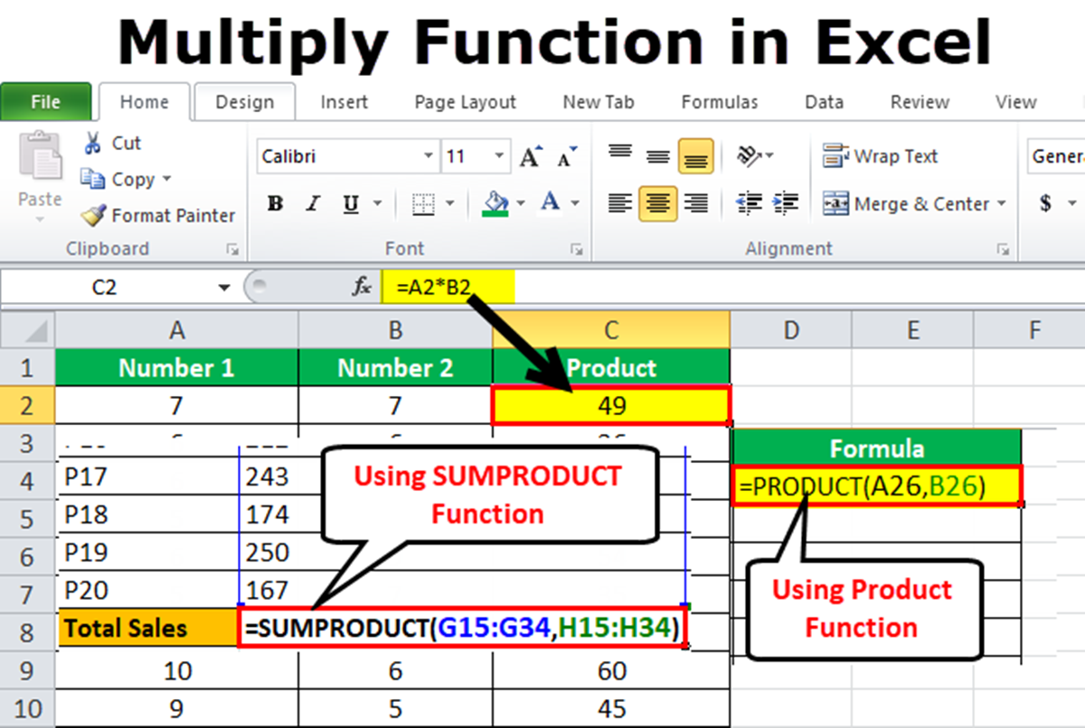
Formulas: To perform multiplication calculations in Excel, you need to use formulas. Formulas in Excel always start with an equal sign (=), followed by the calculation. For multiplication, use the asterisk (*) symbol. For example, “=A1 * B1” multiplies the value in cell A1 by the value in cell B1.
Order of Operations: Excel follows the standard mathematical order of operations, known as BODMAS or PEMDAS. It means that multiplication is performed before addition and subtraction. If you have multiple operations in a formula, consider using parentheses to control the order of calculations.
Cell References: Instead of inputting the actual numbers directly into formulas, you can reference cells that contain the numbers. This allows for easier editing and updating of values. To reference a cell, use the column letter followed by the row number. For example, “A1” refers to cell A1.

Understanding the basics of multiplying in Excel sets the foundation for more advanced calculations. Whether you are calculating sales totals, analyzing data trends, or performing complex financial modeling, multiplication is an essential tool that can save time and ensure accurate results.

Multiplying Numbers in Excel

Excel provides a straightforward way to multiply individual numbers using formulas. Whether you are multiplying small or large numbers, the process remains the same. Here’s how you can multiply numbers in Excel:

Input the Numbers: Start by entering the numbers you want to multiply into separate cells. For example, if you want to multiply 5 by 6, you can enter 5 into cell A1 and 6 into cell B1.
Create a Formula: Next, select an empty cell where you want the multiplication result to appear. Then, enter the formula “=A1 * B1” (without the quotes). This formula multiplies the value in cell A1 by the value in cell B1.
Press Enter: After entering the formula, press the Enter key. Excel will calculate the product by multiplying the two numbers and display the result in the selected cell.

It’s worth noting that Excel allows you to multiply more than two numbers by extending the formula. For example, to multiply 5, 6, and 7, you can use the formula “=5 * 6 * 7”. Excel will multiply all three numbers together and provide the final product.

In addition to using the asterisk (*) operator, you can also use the PRODUCT function to multiply numbers in Excel. The PRODUCT function allows you to multiply a range of numbers without the need to reference each individual cell. To use the PRODUCT function, select an empty cell, enter “=PRODUCT(” and then select the range of numbers you want to multiply, followed by a closing parenthesis.

Multiplying numbers in Excel is a powerful feature that can save time and enhance efficiency in various tasks. From simple calculations to complex data analysis, mastering the art of multiplying numbers in Excel is a valuable skill that every Excel user should possess.

Multiplying Cells in Excel

In Excel, you can go beyond multiplying individual numbers and multiply entire cells. Multiplying cells allows you to perform calculations on a larger scale, such as multiplying rows or columns of data. Here’s how you can multiply cells in Excel:

Select the Target Cell: Start by selecting the cell where you want the product to appear.
Enter the Formula: Next, enter the formula using the asterisk (*) operator. For example, if you want to multiply the values in cells A1 and B1, you can enter the formula “=A1 * B1”.
Press Enter: Once you’ve entered the formula, press the Enter key to calculate the product. Excel will multiply the values in the selected cells and display the result in the target cell.

Excel also allows you to multiply cells across rows or columns by extending the formula. For example, if you want to multiply the values in cells A1, A2, and A3, you can modify the formula to “=A1 * A2 * A3”. Excel will multiply all the values together and provide the final result.

Furthermore, you can use cell references to multiply cells in different locations. Let’s say you want to multiply the values in cells A1 and B2. Instead of inputting the actual values into the formula, you can enter the formula “=A1 * B2”. By using cell references, you can easily update the values in the referenced cells, and the multiplication will automatically recalculate.

When multiplying cells in Excel, it’s important to ensure that the cells contain the correct numerical values. If a cell contains non-numeric data or is empty, Excel will display an error. Make sure to check the cell format and ensure that the data is consistent before performing the multiplication.

Multiplying cells in Excel opens up countless possibilities for performing calculations on large sets of data. Whether you’re working with financial data, inventory management, or statistical analysis, mastering the skill of multiplying cells in Excel can help streamline your workflow and produce accurate results.

Multiplying Ranges in Excel

In Excel, you have the ability to multiply ranges of cells together to perform calculations on a larger scale. Multiplying ranges is particularly useful when working with large datasets or performing calculations across multiple rows or columns. Here’s how you can multiply ranges in Excel:

Select the Target Cell: Begin by selecting the cell where you want the product to appear.
Enter the Formula: Next, enter the formula using the asterisk (*) operator. For example, if you want to multiply all the values in cells A1 to A5, you can enter the formula “=PRODUCT(A1:A5)”.
Press Enter: Once you’ve entered the formula, press the Enter key to calculate the product. Excel will multiply all the values in the selected range and display the result in the target cell.

When multiplying ranges in Excel, you have the flexibility to include multiple columns, rows, or a combination of both. For instance, if you want to multiply the values in cells A1 to C3, you can modify the formula to “=PRODUCT(A1:C3)”. Excel will multiply all the values within the specified range and provide the final result.

It’s important to note that when multiplying ranges, Excel will ignore any non-numeric data or cells that contain text. Therefore, ensure that all the cells within the range contain the appropriate numerical values for accurate multiplication results.

Another useful technique when multiplying ranges is using absolute cell references. Absolute references lock the reference to a specific cell when copying or filling the formula to other cells. By using absolute references, you can ensure that certain cells within the range are always included in the multiplication, regardless of the cell where the formula is copied.

Multiplying ranges in Excel allows for efficient calculations across large sets of data. Whether you’re working with financial models, inventory tracking, or sales forecasts, mastering the skill of multiplying ranges in Excel will enhance your ability to handle complex calculations and produce accurate results.

Using the PRODUCT Function in Excel

In addition to using the asterisk (*) operator, Excel offers a built-in function called PRODUCT that simplifies the process of multiplying values in a range. The PRODUCT function allows you to multiply multiple numbers or cells without the need for using an explicit formula. Here’s how you can use the PRODUCT function in Excel:

Select the Target Cell: Begin by selecting the cell where you want the product to appear.
Enter the Formula: Next, enter the formula using the PRODUCT function. For example, if you want to multiply the values in cells A1 to A5, you can enter the formula “=PRODUCT(A1:A5)”.
Press Enter: Once you’ve entered the formula, press the Enter key to calculate the product. Excel will multiply all the values in the specified range and display the result in the target cell.

The PRODUCT function automatically adjusts to handle a range with either a single column or a single row. If you’re multiplying values across multiple rows and columns, you will need to select the appropriate range in the formula.

Using the PRODUCT function offers several advantages over manual multiplication with the asterisk operator. It simplifies your formulas by eliminating the need to specify individual cells within the range. Additionally, it can save time when dealing with extensive datasets or complex calculations.

One important thing to note is that the PRODUCT function handles empty or non-numeric cells differently than the asterisk operator. It treats empty cells as zeroes, which may affect the multiplication result. Therefore, ensure that the range you’re using with the PRODUCT function doesn’t include any non-numeric data or empty cells that could impact the accuracy of the calculation.

The PRODUCT function is a valuable tool when working with large datasets or extensive calculations that involve multiplying ranges of cells in Excel. By leveraging this function, you can streamline your workflow, reduce the risk of errors, and obtain accurate multiplication results efficiently.

Using Absolute References in Multiplication

When multiplying values in Excel, you may encounter situations where you want to lock certain cells or values in the multiplication formula. This is where absolute references come in. Absolute references allow you to keep specific cell references constant, ensuring that they won’t change when the formula is copied or filled to other cells. Here’s how you can use absolute references in multiplication:

Select the Target Cell: Begin by selecting the cell where you want the product to appear.
Create the Formula: Next, create the multiplication formula using cell references. For example, if you want to multiply cell A1 by cell B1, enter the formula “=A1 * B1”.
Convert to Absolute References: To convert a specific cell reference to an absolute reference, add a dollar sign (‘$’) before the column letter and the row number. For example, to lock cell A1 as an absolute reference, change the formula to “=$A$1 * B1”.
Copy the Formula: Copy or fill the formula to other cells as needed. The absolute reference will ensure that cell A1 remains constant in all the multiplication calculations, even if the formula is pasted to different cells.

Absolute references are particularly useful when you want to multiply a range of cells by a specific value or when performing calculations across different rows or columns. By using absolute references, you can easily apply the multiplication formula to different cells without the need to manually adjust the references each time.

Furthermore, absolute references can also be applied to rows or columns within a range. For example, if you want to lock column A but allow the row number to change, you can use the formula “=$A1 * B1”. This will fix the column reference to column A while allowing the row to vary based on the cell where the formula is copied or filled.

Using absolute references in multiplication provides greater control over the cells and values involved in the calculation. It ensures accuracy and consistency when dealing with complex formulas or large datasets. By mastering the skill of applying absolute references in multiplication, you can effectively manipulate and analyze data in Excel.

Multiplying Numbers with Negative Values in Excel

In Excel, multiplying numbers is a straightforward task, but when it comes to working with negative values, there are a few key considerations to keep in mind. Understanding how Excel handles negative values during multiplication is crucial for accurate calculations. Here’s what you need to know when multiplying numbers with negative values in Excel:

When multiplying a positive number by a negative number, the resulting product will be negative. For example, if you multiply 5 by -2, the result will be -10.

Similarly, when multiplying two negative numbers, the result will be positive. For instance, if you multiply -3 by -4, the product will be 12.

It’s important to note that Excel follows the standard mathematical rules for multiplication, where the product of two negative numbers is always positive. However, if you specifically want to keep the negative sign in the result, you can use parentheses to indicate the multiplication.

For example, if you want to multiply -5 by 3 and keep the negative sign, you can use the formula “=(-5) * 3”. Excel will calculate the product as -15.

When working with more complex formulas involving both positive and negative numbers, it’s crucial to consider the order of operations using parentheses and follow the general mathematical rules for multiplication. Properly structuring a formula ensures that Excel performs the calculations correctly and provides accurate results.

In some cases, you may encounter scenarios where you want to multiply a negative number by a range of cells or a range of negative numbers. In these situations, Excel will automatically apply the multiplication rules discussed above, resulting in the appropriate positive or negative product.

Understanding how Excel handles negative values during multiplication allows you to perform accurate calculations and obtain the correct results. By applying the proper formula structure and considering the order of operations, you can make the most of Excel’s features when working with negative values in multiplication.

Applying Conditional Formatting to Multiplication Results in Excel

In Excel, conditional formatting is a powerful tool that allows you to visualize and highlight specific patterns or conditions within your data. By applying conditional formatting to multiplication results, you can easily identify certain values or ranges that meet specific criteria. Here’s how you can utilize conditional formatting to enhance your multiplication results in Excel:

Select the Result Range: Start by selecting the range of cells where the multiplication results will appear.
Click on Conditional Formatting: Go to the “Home” tab on the Excel ribbon and locate the “Conditional Formatting” button.
Choose a Formatting Rule: From the drop-down menu, select the desired formatting rule. For example, you can choose “Highlight Cells Rules” and then “Greater Than” to highlight values that are greater than a specific threshold.
Specify the Condition: Enter the threshold or criteria for the condition in the input box. This could be a specific number or a reference to another cell with the threshold value.
Select the Formatting Style: Choose the formatting style, such as font color, background color, or cell border, to apply to the cells that meet the specified condition.
Click OK: Once you’ve set up the formatting rule and style, click OK to apply the formatting to the multiplication results.

By applying conditional formatting, you can easily identify which multiplication results meet specific requirements or stand out from the rest of the data. This can be particularly useful when analyzing large datasets or performing complex calculations where certain values need to be highlighted.

Moreover, conditional formatting can be used with various criteria, such as highlighting values that are equal to, not equal to, greater than, or less than a particular threshold. You can customize the formatting rules to suit your specific needs and adjust them as necessary.

Conditional formatting is a powerful feature in Excel that allows you to visually enhance your multiplication results. By using conditional formatting, you can quickly identify important patterns or trends in your data and make data analysis more efficient and effective.

Using the Fill Handle to Multiply in Excel

In Excel, the fill handle is a convenient tool that allows you to quickly fill a series of cells with a pattern or sequence. When it comes to multiplication, the fill handle can save you time and effort by automatically extending your multiplication formula to adjacent cells. Here’s how you can use the fill handle to multiply in Excel:

Enter the Initial Multiplication: Start by entering your multiplication formula into the first cell where you want the calculation to begin. For example, you can input “=A1 * B1” into cell C1.
Select the Cell with the Formula: Click on the cell with the multiplication formula to select it.
Drag the Fill Handle: Move your cursor over the fill handle, which is the small square in the bottom right corner of the selected cell. The cursor should turn into a plus sign (+).
Drag the Fill Handle Down or Across: While holding down the left mouse button, drag the fill handle down to fill the formula into the cells below or drag it across to fill the formula into the cells to the right.
Release the Mouse Button: Once you’ve dragged the fill handle to the desired range, release the mouse button. Excel will automatically populate the adjacent cells with the appropriate multiplication results.

Excel intelligently adjusts the cell references in the multiplication formula as you use the fill handle. For example, if you drag the fill handle down, Excel will automatically change the cell references to match the corresponding rows. If you drag the fill handle across, Excel will adjust the cell references to match the corresponding columns.

The fill handle is an efficient way to perform repetitive multiplications in Excel, especially when you have a large dataset or need to extend your calculations to multiple rows or columns. It eliminates the need to manually input formulas into each cell and saves you valuable time and effort.

Additionally, the fill handle can be used with other types of calculations in Excel, such as addition, subtraction, or division. It has a wide range of applications and can greatly streamline your data entry and calculation processes.