
Getting Started with Adding Numbers in Excel
Excel is a powerful spreadsheet software that allows you to perform various calculations, including adding numbers. Whether you are a beginner or have some experience with Excel, understanding how to add numbers using formulas is an essential skill that can significantly improve your productivity.
Before we dive into the specifics of adding numbers in Excel, it’s important to understand the basics of Excel formulas. In Excel, formulas are used to perform calculations and can be created by combining numbers, operators, and functions. Formulas always begin with an equal sign (=) to indicate that it is a formula.
To add numbers in Excel, you can either use basic arithmetic formulas or built-in functions. Arithmetic formulas involve using operators like plus (+), minus (-), multiply (*), and divide (/) to perform calculations. On the other hand, built-in functions, such as the SUM function, provide a quicker and more efficient way to add numbers.
The most straightforward way to add numbers in Excel is by using the addition (+) operator. Simply select the cell where you want the sum to appear and enter the formula using the following format: “=A1 + A2”. This formula adds the values in cells A1 and A2. You can adjust the cell references according to your specific data arrangement.
Another useful method for adding numbers in Excel is by utilizing the SUM function. The SUM function allows you to add multiple numbers or a range of cells. To use the SUM function, select the cell where you want the sum to appear and enter the formula using the format: “=SUM(A1:A5)”. This formula adds the values in cells A1 through A5.
If you want to add numbers across multiple sheets in Excel, you can use the same formulas or functions, but with the addition of sheet names and exclamation marks. For example, “=Sheet1!A1 + Sheet2!A1” adds the values in cell A1 from Sheet1 and cell A1 from Sheet2.
An even quicker way to add numbers in Excel is by using the AutoSum feature. This feature automatically detects a range of adjacent cells and inserts the SUM function for you. Simply select the cell where you want the sum to appear and click the AutoSum button in the toolbar.
Excel also allows you to add numbers with decimal places or add negative numbers. When adding numbers with decimal places, make sure to match the decimal formatting of the cells. For negative numbers, you can use the minus (-) operator or enter the number with a negative sign.
Lastly, Excel allows you to customize the number format to suit your needs. You can choose to display currency symbols, thousands separators, or specify the number of decimal places. Simply select the cells containing the numbers and adjust the number formatting settings in the toolbar.
By mastering the art of adding numbers in Excel, you can streamline your calculations and improve your efficiency in handling data. Practice these techniques and explore more advanced functions to take your Excel skills to the next level.
Understanding Excel Formulas
Excel formulas are the backbone of any spreadsheet. They allow you to perform calculations, manipulate data, and automate tasks. Having a thorough understanding of Excel formulas is crucial for maximizing the power and efficiency of this versatile software.
At its core, an Excel formula is an equation that starts with an equal sign (=) and performs a mathematical operation or a logical function. Formulas can consist of numbers, cell references, operators, and functions.
Cell References: In Excel, cell references are used to refer to specific cells within a spreadsheet. They are denoted by a combination of the column letter and row number, such as A1 or B3. Cell references allow you to dynamically update formulas when the referenced cells’ values change.
Operators: Excel supports a variety of operators to perform different mathematical operations. These include the plus sign (+) for addition, minus sign (-) for subtraction, asterisk (*) for multiplication, forward slash (/) for division, and caret (^) for exponentiation. Operators can be combined within a formula to create complex calculations.
Functions: Excel provides a vast library of built-in functions that perform specific calculations. Functions can simplify complex calculations and save time. Some commonly used functions include SUM for adding a range of numbers, AVERAGE for calculating the average, MAX for finding the maximum value, and MIN for finding the minimum value.
Formulas in Action: Let’s take a simple example to understand how formulas work. Suppose we have a column of numbers in cells A1 to A5, and we want to calculate the total sum. We can use the SUM function by entering “=SUM(A1:A5)” in a different cell. Excel will calculate and display the sum of the values in cells A1 to A5.
Formula Errors: It’s important to be aware of common formula errors that may occur in Excel. These errors can happen due to incorrect syntax, referencing empty cells, divided by zero, or other issues. Excel provides error checking tools and error-handling functions to help identify and troubleshoot formula errors.
Using Formulas Across Sheets: Excel allows you to use formulas across multiple sheets or workbooks. To reference a cell on a different sheet, include the sheet name followed by an exclamation mark (!) before the cell reference. For example, “Sheet2!A1” refers to cell A1 on Sheet2.
As you become more comfortable with Excel formulas, you can explore more advanced features like conditional formulas, nested formulas, and array formulas. These advanced techniques can provide powerful solutions for complex calculations.
Understanding Excel formulas is essential for harnessing the full potential of this software. By leveraging formulas, you can automate repetitive tasks, analyze data efficiently, and make informed decisions based on accurate calculations. Take the time to explore and practice different formulas, and you’ll soon become proficient in using Excel to its fullest extent.
Basic Arithmetic Formulas in Excel
Excel is renowned for its ability to perform complex calculations, but it is equally capable when it comes to basic arithmetic. Using simple arithmetic formulas, you can add, subtract, multiply, and divide numbers in Excel, just like you would with a calculator.
The basic arithmetic operators in Excel include:
- Plus (+): Used for addition
- Minus (-): Used for subtraction
- Asterisk (*): Used for multiplication
- Forward slash (/): Used for division
To use these operators in Excel, you’ll need to start your formula with an equal sign (=). Let’s take a look at some examples:
Addition: To add numbers, use the plus (+) operator. For instance, if you want to add the values in cells A1 and A2, the formula would be “=A1 + A2”. This will calculate the sum and display the result in the cell where the formula is entered.
Subtraction: To subtract numbers, use the minus (-) operator. For example, if you want to subtract the value in cell B1 from the value in cell B2, the formula would be “=B2 – B1”. Excel will perform the subtraction and show the result in the formula cell.
Multiplication: To multiply numbers, use the asterisk (*) operator. If you want to multiply the values in cells C1 and C2, the formula would be “=C1 * C2”. Excel will multiply the two numbers and display the product.
Division: To divide numbers, use the forward slash (/) operator. For example, if you want to divide the value in cell D1 by the value in cell D2, the formula would be “=D1 / D2”. Excel will perform the division and show the quotient.
Note that Excel follows the general rules of arithmetic when it comes to the order of operations. This means that calculations are performed from left to right, respecting the hierarchy of operators. However, you can use parentheses to override the default order of operations and prioritize certain calculations.
Furthermore, Excel allows you to combine multiple operators within a single formula. For example, you can create a formula that adds two numbers, multiplies the result by a third number, and subtracts yet another number.
By mastering basic arithmetic formulas in Excel, you can perform quick and accurate calculations, saving time and effort. Whether you’re managing personal finances, tracking expenses, or analyzing data, understanding these arithmetic formulas is a fundamental skill that will serve you well in Excel.
Addition Formulas in Excel
When it comes to adding numbers in Excel, you have a range of options at your disposal. Excel provides various formulas and functions that allow you to add numbers quickly and efficiently, catering to different data arrangements and requirements.
The most straightforward way to add numbers in Excel is by using basic arithmetic formulas. You can utilize the plus (+) operator to indicate the addition operation between two or more numbers. For example, if you want to add the values in cells A1 and A2, you can use the formula “=A1 + A2”. Excel will calculate the sum and display the result in the formula cell.
Excel also offers built-in functions that simplify the process of adding numbers. One of the most commonly used functions for addition is the SUM function. This function allows you to add multiple numbers or a range of cells effortlessly. To use the SUM function, select the cell where you want the sum to appear and enter the formula using the format “=SUM(A1:A5)”. This formula adds the values in cells A1 through A5 and displays the total sum.
The SUM function can also be used with non-adjacent cells by specifying multiple ranges. For example, “=SUM(A1:A5, C1:C3)” adds the values in cells A1 to A5 as well as C1 to C3. This flexibility enables you to add numbers from different parts of your spreadsheet easily.
Another useful way to add numbers in Excel is by using the AutoSum feature. The AutoSum button, conveniently located in the toolbar, automatically detects a range of adjacent cells and inserts the SUM function for you. Simply select the cell where you want the sum to appear and click the AutoSum button. Excel will populate the cell with the SUM formula, including the appropriate range of cells.
Excel goes beyond basic addition by allowing you to add numbers across multiple sheets. This can be achieved by referencing cells from different sheets in your formulas. For example, if you want to add the value in cell A1 from Sheet1 to the value in cell B2 from Sheet2, you can use the formula “=Sheet1!A1 + Sheet2!B2”. Excel will fetch the respective values from the specified sheets and calculate the sum.
Adding numbers in Excel becomes even more convenient when you employ keyboard shortcuts. For instance, to quickly add the values in a column, select an empty cell below the column of numbers, hold down the Alt key, and press the equal (=) key. Excel will automatically generate the SUM formula, saving you time and effort.
By leveraging the addition formulas and functions in Excel, you can perform accurate calculations and obtain the desired sum of numbers. Whether you prefer using basic arithmetic formulas or the flexibility of built-in functions, Excel provides you with the tools to add numbers efficiently and effectively.
The SUM Function in Excel
When it comes to calculating the total sum of a range of numbers in Excel, one of the most powerful and versatile functions to use is the SUM function. The SUM function allows you to add multiple numbers or a range of cells with ease, providing you with accurate and efficient results.
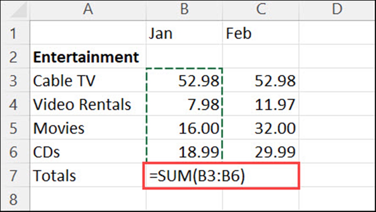
The syntax of the SUM function is straightforward. To utilize the SUM function, select the cell where you want the sum to appear and enter the formula “=SUM(range)”. The “range” can be a collection of individual cells or a continuous range of cells. For example, if you want to add the numbers in cells A1, A2, and A3, the formula would be “=SUM(A1:A3)”. Excel will calculate the sum and display the result in the cell.
The beauty of the SUM function lies in its ability to handle large data sets. Instead of manually entering each cell reference, you can specify the entire range using the colon (:) separator. This saves time and reduces the chances of manual errors in calculating the sum.
Excel’s SUM function is not limited to a single range of cells. It can handle multiple ranges as well. Simply separate each range with a comma (,). For example, if you want to add the values in cells A1:A5 and C1:C3, the formula would be “=SUM(A1:A5, C1:C3)”. Excel will calculate the sum of the numbers in both ranges and display the total sum.
In addition to numeric values, the SUM function in Excel is also capable of handling other types of data. It automatically ignores any non-numeric values within the range, allowing you to perform calculations without worrying about errors caused by text or empty cells.
Another useful feature of the SUM function is its compatibility with formulas and functions. You can include formulas or nested functions within the range you specify for the SUM function. Excel will evaluate these formulas or functions first, and then calculate the sum based on the results. This enables you to create more complex calculations and achieve dynamic sums.
Excel also provides a quick and convenient way to use the SUM function with the AutoSum feature. You can simply select the cell where you want the sum to appear and click the AutoSum button in the toolbar. Excel will automatically detect the contiguous range of cells above or to the left of the selected cell and insert the SUM formula for you.
The SUM function in Excel is a powerful tool for adding numbers and performing calculations with ease. It eliminates the need for manual calculations, saves time, and ensures accuracy in your data analysis. By mastering the SUM function, you can handle large data sets efficiently and obtain accurate sums with a few simple steps.
Summing a Range of Cells in Excel
Excel offers several methods to sum a range of cells, allowing you to quickly calculate the total of a selected set of numbers. Whether you’re working with a small range or a large dataset, Excel provides flexible options to sum numeric values efficiently.
One way to sum a range of cells in Excel is by using the SUM function. To do this, select the cell where you want the sum to appear and enter the formula “=SUM(range)”. Replace “range” with the desired cell range you want to sum. For example, if you want to sum the values in cells A1 to A5, the formula would be “=SUM(A1:A5)”. Excel will calculate the sum and display the result in the cell.
In addition to using the SUM function, you can also utilize the AutoSum feature to sum a range of cells quickly. Select an empty cell next to the range you want to sum, and click the AutoSum button in the toolbar. Excel will automatically detect the contiguous range of cells above or to the left of the selected cell and insert the SUM formula for you. Press Enter to calculate the sum.
Another practical method for summing a range of cells in Excel is by manually selecting the range. Simply click and drag the cursor over the desired cells to highlight them. Excel will display the sum of the selected cells in the Status Bar, located at the bottom of the Excel window. You can also customize the calculation displayed in the Status Bar by right-clicking on it and selecting the desired calculation option, such as Sum, Average, Minimum, or Maximum.
If you want to keep track of the sum of a range of cells as you update the data within the range, you can use the Formula Bar. Select the cell where you want the sum to appear and enter the formula “=SUM(“. Then, click and drag the cursor over the cells you want to include in the sum. Close the formula with a closing parenthesis, and press Enter to calculate the sum.
Excel also offers a useful shortcut for summing a range of cells. After selecting the range, look at the bottom-right corner of the Excel window. You will see the sum of the selected cells displayed in the status bar, preceded by the word “Sum”. By default, Excel displays the sum, but you can customize the calculation by right-clicking on it and selecting a different option.
Summing a range of cells in Excel is a crucial tool for data analysis and numerical calculations. Whether you choose to use the SUM function, AutoSum, the Formula Bar, or the Status Bar, Excel provides multiple options to suit your needs. By mastering these techniques, you can efficiently and accurately sum ranges of cells and streamline your data analysis process.
Adding Numbers Across Multiple Sheets in Excel
Excel provides a powerful capability to work with multiple sheets within a workbook. When you need to add numbers from different sheets, Excel allows you to easily combine and calculate the total sum across those sheets. Whether you have data on two sheets or even more, Excel offers several methods to make adding numbers across multiple sheets a seamless process.
One way to add numbers from different sheets in Excel is by using the plus (+) operator along with sheet references. Simply select the cell where you want the sum to appear and enter the formula “=Sheet1!A1 + Sheet2!B1”. This formula adds the value in cell A1 from Sheet1 to the value in cell B1 from Sheet2, and Excel displays the sum in the selected cell. You can adjust the sheet names and cell references according to your specific workbook structure.
If you have a large dataset across multiple sheets and want to sum values from the same cell across each sheet, you can use the SUM function with sheet references. For example, to add the values in cell A1 from Sheet1 to Sheet3, you can use the formula “=SUM(Sheet1:Sheet3!A1)”. Excel will calculate the sum across the specified sheets and display the result.
Another method to add numbers across multiple sheets in Excel is by using the SUM function along with explicit references to cell ranges on each sheet. For example, if you want to add the values in cells A2 to A5 from Sheet1 to Sheet3, you can use the formula “=SUM(Sheet1!A2:A5, Sheet2!A2:A5, Sheet3!A2:A5)”. Excel will calculate the sum of the specified ranges on each sheet and provide the total sum.
If you have a large number of sheets and want to sum values from all sheets in your workbook, you can utilize the SUM function along with the INDIRECT function. The INDIRECT function allows you to dynamically create a cell reference based on a text string. For example, you can use the formula “=SUM(INDIRECT(“Sheet1:Sheet”&A1&”!A1″))”. By entering the sheet numbers in cells A1, A2, A3, and so on, Excel will dynamically create the cell references and sum the values from those sheets.
Excel also offers a convenient way to navigate between sheets and select cell ranges for summing. Hold down the Ctrl key on your keyboard and click on the sheet tabs that you want to include in the calculation. This allows you to quickly select multiple sheets, and then enter the appropriate SUM formula in the desired cell to obtain the sum of the selected ranges across the sheets.
By harnessing the features and formulas available in Excel, you can easily add numbers from different sheets and calculate the total sum across multiple sheets within a workbook. These methods enable you to streamline your data analysis and obtain accurate results when working with complex datasets.
Using AutoSum to Add Numbers in Excel
Excel provides a quick and effortless way to add numbers with the AutoSum feature. This powerful feature automatically detects the range of cells you want to add and inserts the appropriate sum formula for you. By utilizing AutoSum, you can save time and eliminate the need for manual entry of formulas.
To use AutoSum, first, select the cell where you want the sum to appear. Then, locate the AutoSum button in the toolbar. The button looks like the Greek letter sigma (∑). It is typically located in the Home tab or the Formulas tab, depending on your version of Excel.
Once you click the AutoSum button, Excel will automatically detect a range of adjacent cells that it believes you want to add. It highlights the range with a dotted line or a marquee, and inserts the SUM formula in the selected cell. Press Enter to calculate the sum and display the result.
AutoSum is not limited to just a single row or column. It can be used to sum a range of cells in any direction. For example, if you want to sum a row of numbers, select an empty cell at the end of the row and click the AutoSum button. Excel will detect the adjacent cells in that row and insert the sum formula accordingly. Likewise, if you want to sum a column of numbers, select an empty cell below the column and click the AutoSum button.
If you want to make adjustments to the range selected by AutoSum, simply click and drag the cursor to modify the range. Excel will automatically update the sum formula to reflect the new selected range, allowing you to fine-tune the calculation as needed.
AutoSum can also be used to add numbers from multiple columns or rows. Simply select the range of cells that you want to sum, and then click the AutoSum button. Excel will insert the sum formula encompassing the selected range, providing you with the total sum across the chosen columns or rows.
Furthermore, AutoSum can handle non-adjacent ranges. Hold down the Ctrl key on your keyboard and select multiple non-adjacent ranges, and then click the AutoSum button. Excel will automatically insert multiple sum formulas, each representing the sum of the individual selected ranges.
AutoSum is a versatile tool that allows you to add numbers quickly and accurately in Excel. By leveraging this feature, you can streamline your data analysis, save time, and reduce the chances of manual errors in your calculations. AutoSum is a valuable aid for anyone working with numbers in Excel, from beginners to experienced users.
Adding Numbers with Decimal Places in Excel
When working with numbers in Excel, it’s important to accurately account for decimal places. Excel provides various methods to add numbers with decimal places, allowing you to perform precise calculations and maintain the desired level of precision in your data analysis.
To add numbers with decimal places in Excel, simply enter the values with the appropriate decimal formatting. For example, if you want to add the numbers 3.14 and 2.75, enter them as 3.14 and 2.75, respectively, in the cells. When you use the plus (+) operator or the SUM function to add these values, Excel will automatically account for the decimal places and display the correct sum.
If you have a range of cells with decimal values that you want to add, you can utilize the SUM function. Select the cell where you want the sum to appear and enter the formula “=SUM(A1:A5)”, adjusting the range (A1:A5) according to your specific data. Excel will calculate the sum and display it with the appropriate decimal places.
Excel also offers the flexibility to adjust the decimal places displayed in your calculations. By default, Excel displays two decimal places for most numbers. However, you can customize this formatting based on your preferences or specific data requirements.
To customize the number formatting, select the cells containing the numbers you want to adjust. Right-click and choose “Format Cells” from the context menu. In the Format Cells dialog box, go to the Number tab. Here, you can choose the desired category, such as Number, Currency, or Accounting, and specify the number of decimal places you want to display.
If you want to set a consistent decimal place format for all numbers in your workbook, you can modify the default settings in Excel. Go to File > Options > Advanced. Scroll down to the “Editing Options” section and find the option for “Automatically insert a decimal point.” Tick the box and specify the number of decimal places you prefer.
When adding numbers with different decimal places, Excel retains the precision of the calculated result. This means that if you add two numbers with different decimal places, the sum will maintain the highest level of precision. For example, if you add 2.2 and 3.1415, the result will be displayed as 5.3415.
Excel’s ability to handle decimal places accurately is crucial for tasks such as financial calculations, scientific data analysis, and inventory management. By understanding and utilizing the various options available for handling decimal places in Excel, you can ensure the integrity and precision of your calculations.
Adding Negative Numbers in Excel
In Excel, adding negative numbers is just as simple as adding positive numbers. Excel’s arithmetic operations can handle negative values with ease, allowing you to perform accurate calculations and analyze data that includes both positive and negative numbers.
To add negative numbers in Excel, use the minus (-) operator as you would for subtraction or use the negative sign (-) directly in front of the number. For example, if you want to add -5 and -3, you can enter the formula “= -5 + (-3)”. Excel will perform the addition operation and display the result, which in this case would be -8.
If you have a range of cells with negative values that you want to add, you can utilize the SUM function. Select the cell where you want the sum to appear and enter the formula “=SUM(A1:A5)”, adjusting the range (A1:A5) to match your specific data. Excel will calculate the sum, taking into account the negative numbers, and display the result accordingly.
When adding both positive and negative numbers in Excel, ensure you use the appropriate sign for each value. For positive numbers, prefix them with a plus (+) sign, although it is not mandatory. For negative numbers, either enter the negative sign (-) directly in front of the number or enclose the number in parentheses with a negative sign. For example, you can enter “+5” for a positive number or “-5” or “(5)” for a negative number.
Excel’s flexibility with negative numbers extends to formulas and functions as well. You can incorporate negative numbers within complex calculations, nested formulas, and even within functions like SUM. Excel will accurately evaluate the formulas and functions, ensuring the correct addition of both negative and positive numbers.
Excel also provides formatting options to distinguish negative numbers visually. By default, Excel uses a minus sign (-) to represent negative numbers. However, you can customize the formatting to display negative numbers in different ways. Right-click on the cell or range of cells, select “Format Cells,” and choose the desired format from the Number tab.
The ability to add negative numbers in Excel is particularly useful in finance, accounting, and other scenarios where debits and credits, expenses and incomes, and gains and losses need to be accounted for. By leveraging Excel’s capabilities, you can perform precise calculations, maintain accuracy in your data analysis, and confidently work with negative numbers in your spreadsheets.
Adding Text and Numbers in Excel
In Excel, you can combine text and numbers together to create more meaningful and informative data. This allows you to add context to your numerical values or create labels that enhance the understanding and interpretation of your data.
When adding text and numbers in Excel, you can simply use the ampersand (&) operator to concatenate, or join, the text and number. For example, if you have a number in cell A1 and want to combine it with a piece of text in cell B1, you can use the formula ” =B1 & A1″. This formula joins the contents of cell B1 and the value in cell A1 into a single cell, displaying the combined result.
If you want to add a space or any other characters between the text and number, you can incorporate them within double quotation marks. For instance, if you want to add a space between the text and number, you can use the formula ” =B1 & ” ” & A1″. This formula will combine the contents of cell B1, a space, and the value in cell A1, displaying the concatenated result with the desired spacing.
In addition to using the ampersand operator, Excel provides another option for combining text and numbers called the CONCATENATE function. The CONCATENATE function takes multiple text and number arguments and joins them together. For example, the formula “=CONCATENATE(B1, ” “, A1)” will concatenate the content of cell B1, a space, and the value in cell A1, producing the desired combined result.
Excel also allows you to perform calculations on numbers that are combined with text. If you have a numeric value within the text string, you can extract the number and use it for arithmetic operations. You can achieve this by utilizing functions like VALUE or LEFT/RIGHT/MID to extract the numerical part from the text and perform necessary calculations.
It’s important to note that when combining text and numbers in Excel, the result will be treated as text. Thus, you won’t be able to perform mathematical operations directly on the combined result unless you extract the numbers using appropriate functions.
Adding text and numbers in Excel is particularly useful when working with labels or creating customized report outputs. It allows you to present data in a more organized and meaningful manner, providing clearer insights and improving data interpretation.
By leveraging the ability to add text and numbers in Excel, you can enhance the quality and effectiveness of your spreadsheets, making them more informative and visually appealing.
Customizing the Number Format in Excel
Excel offers a variety of options for customizing the number format, allowing you to display your numerical data in different formats based on your specific needs and preferences. By customizing the number format, you can enhance readability, highlight important values, and format numbers as percentages, currencies, or with specific decimal places.
To change the number format in Excel, select the cells or range of cells that you want to format. Right-click and choose “Format Cells” from the context menu. In the Format Cells dialog box, go to the Number tab. Here, you’ll find a wide range of formatting categories, such as Number, Currency, Accounting, Percentage, Date, and more.
Let’s explore some of the customization options available in Excel:
- Decimal Places: If you want to display numbers with a specific number of decimal places, select the “Number” category and choose the desired decimal places. You can increase or decrease decimal places to suit your requirements.
- Currency Format: When dealing with financial data, the currency format is handy. Select the “Currency” category and choose the currency you want to use. Excel will automatically format the numbers with the appropriate currency symbol and decimal places.
- Percentage Format: Use the “Percentage” category to format numbers as percentages. Excel will automatically multiply the value by 100 and add the percentage sign. This is great for displaying growth rates, ratios, or any data that represents a percentage.
- Thousands Separators: To make large numbers more readable, you can choose to include thousands separators. This adds commas or periods to separate the digits into groups of thousands. Select the “Number” category and choose the desired thousands separator option.
- For example, if you want to format the number 100000 as 100,000, select the “Number” category and choose the appropriate thousands separator option.
- Negative Number Format: You can customize how negative numbers are displayed in Excel. For example, you can choose to display negative numbers in red or in parentheses. To customize the negative number format, go to the “Number” category and specify the desired format in the “Negative numbers” section.
Excel also allows you to create and apply custom number formats using the “Custom” category. This allows for greater flexibility and control. You can define your own format codes and apply them to specific cells or ranges. Custom number formats are especially useful when you have specific formatting requirements or when you want to display numbers in a unique way.
By customizing the number format in Excel, you can effectively present numerical data in a visually appealing and meaningful way. Whether you want to display decimal places, format as currency or percentages, or apply custom formats, Excel provides extensive options to meet your formatting needs.