
What is the CONCATENATE Function in Excel?
The CONCATENATE function in Excel is a powerful tool that allows you to combine the contents of multiple cells into a single cell. It is especially useful when working with large datasets or when you need to create custom labels or reports. By using the CONCATENATE function, you can easily merge text, numbers, or a combination of both, making it a versatile function for various applications in Microsoft Excel.
The CONCATENATE function in Excel joins multiple text strings together. It takes one or more text values as input and returns a new text string that is the combination of these input values. The function can be used to merge cells from the same worksheet or even from different worksheets in a workbook.
The CONCATENATE function syntax in Excel is straightforward. It requires specifying the text strings or cell references you want to combine, separated by commas. The function also allows you to add custom characters or spaces between the merged values.
By utilizing the CONCATENATE function, you can streamline your data manipulation tasks and create more efficient spreadsheets. It eliminates the need for manual copying and pasting, allowing you to save time and reduce potential errors. Whether you are preparing reports, generating unique IDs, or creating personalized messages, the CONCATENATE function is a valuable tool that helps you achieve your desired results in Excel.
Syntax of the CONCATENATE Function
The syntax of the CONCATENATE function in Excel is quite simple and easy to understand. It follows a specific format:
=CONCATENATE(text1, text2, …)
The CONCATENATE function begins with an equal sign followed by the word CONCATENATE. Inside the parentheses, you specify the text strings or cell references that you want to join together. You can include as many arguments as you need, separated by commas. Each argument can be a text string enclosed in double quotation marks or a cell reference containing text.
For example, if you want to combine the contents of cell A1 and B1, the formula would be:
=CONCATENATE(A1, B1)
This formula would merge the values of cell A1 and B1 into a single cell.
In addition to combining text strings, the CONCATENATE function can also handle the combination of numbers or a mix of text and numbers. Excel automatically converts numbers to text during the concatenation process.
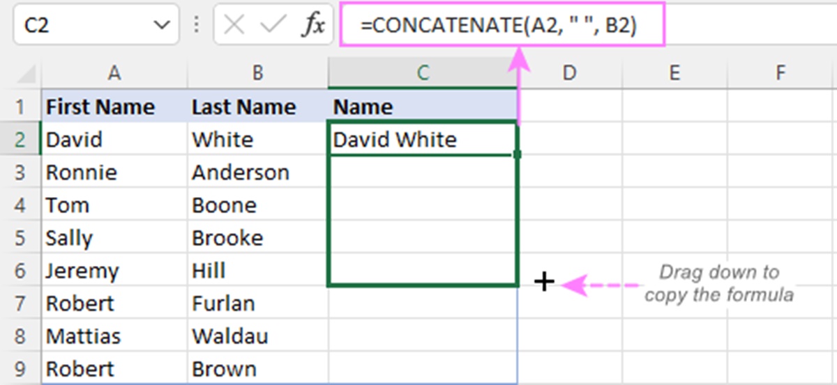
You can also include additional custom characters or spaces between the concatenated values by inserting them as text within double quotation marks. For instance, to add a space between the merged values, the formula would be:
=CONCATENATE(A1, ” “, B1)
This formula would join the values of cell A1, a space, and the value of cell B1, resulting in a cell with the merged text.
It’s important to note that while the CONCATENATE function is very powerful, it can become cumbersome when dealing with a large number of cells. In such cases, using other functions like CONCAT or the ampersand (&) operator may be more efficient.
Using the CONCATENATE Function to Combine Cells
The CONCATENATE function in Excel allows you to easily combine the contents of multiple cells into a single cell. This can be especially useful when you want to create unique labels, generate custom reports, or merge data for analysis. By using the CONCATENATE function, you can save time and effort by automating the process of combining cell values.
To use the CONCATENATE function, you simply need to specify the cell references or text strings you want to merge. Here’s how you can do it:
- Select the cell where you want the merged result to appear.
- Type the CONCATENATE formula with the desired cell references or text strings enclosed in parentheses, separated by commas.
- Press Enter to see the combined result in the chosen cell.
For example, let’s say you have two cells, A1 and A2, containing the values “Hello” and “World” respectively. To combine these cells, you can use the CONCATENATE function as follows:
=CONCATENATE(A1, A2)
Upon entering the formula, the merged result “HelloWorld” will appear in the designated cell.
In addition to combining adjacent cells, you can also merge cells from different worksheets by referencing them in the CONCATENATE formula. For example, if you want to combine cell A1 from Sheet1 and cell B2 from Sheet2, you can use the following formula:
=CONCATENATE(Sheet1!A1, Sheet2!B2)
This formula will merge the values from the specified cells across different worksheets into a single cell.
By utilizing the CONCATENATE function, you can easily merge cell values and create customized output in Excel. Whether you’re working with small datasets or large spreadsheets, this function provides a straightforward way to combine cells and streamline your data manipulation tasks.
Combining Text and Numbers with CONCATENATE
The CONCATENATE function in Excel is not limited to combining text strings; it can also seamlessly merge text and numeric values. This flexibility makes it a powerful tool for creating custom labels, unique identifiers, or generating reports that include both textual and numerical information.
To combine text and numbers using the CONCATENATE function, you need to ensure that the numeric values are formatted as text. Excel automatically converts numbers to text when they are included in the CONCATENATE function.
Here’s an example of how you can use CONCATENATE to combine text and numbers:
- Type the desired text string or label in quotation marks, followed by a comma.
- Add the cell reference containing the numeric value or use the desired number directly.
- Repeat for additional text and numeric values, separating them with commas.
For instance, if you have the text “Product #” and a numeric value in cell A1, you can use the CONCATENATE function as follows:
=CONCATENATE(“Product #”, A1)
This formula will merge the text “Product #” with the value in cell A1, resulting in a combined output. If cell A1 contains the number 123, the merged result will be “Product #123”.
You can also add other text strings or characters to further enhance the merged output. For example:
=CONCATENATE(“Product #”, A1, ” – Available”)
This formula will merge the text “Product #”, the value in cell A1, and the text ” – Available”. If cell A1 contains the number 123, the merged result will be “Product #123 – Available”.
By incorporating numeric values into your CONCATENATE formulas, you can create dynamic and informative labels or reports that combine both text and numbers. Whether you need to generate unique identifiers, product codes, or summary reports, the CONCATENATE function provides a versatile solution for merging text and numeric values in Excel.
Adding Space or Other Characters between Cells
The CONCATENATE function in Excel not only allows you to combine cells, but it also provides the flexibility to add custom characters or spaces between the merged values. This feature can be particularly useful when you want to create a specific formatting or formatting for your merged output, such as adding a separator or delimiter between the combined cell values.
To add space or other characters between cells using the CONCATENATE function, you simply need to include them as text within double quotation marks in the formula. Here’s how you can do it:
- Type the desired text string or character in quotation marks, followed by a comma.
- Add the first cell reference or text string that you want to merge.
- Repeat the process for additional cells or text strings, separating them with commas.
For example, let’s say you have the values “Apple” in cell A1 and “Banana” in cell B1, and you want to merge them with a space in between. You can use the CONCATENATE function as follows:
=CONCATENATE(A1, ” “, B1)
This formula will combine the values in cell A1 and B1, with a space character in between. The merged result will be “Apple Banana”.
You can add any character or string within the quotation marks to act as a separator. For instance, if you prefer a comma as a separator, the formula would be:
=CONCATENATE(A1, “, “, B1)
This formula will merge the values in cell A1 and B1, with a comma and space in between. The merged result will be “Apple, Banana”.
By utilizing custom characters or spaces between cells, you can customize the formatting and appearance of your merged output. Whether you want to add separators, special characters, or special formatting, the CONCATENATE function empowers you to create the desired output with ease and efficiency in Excel.
Using CONCATENATE with Multiple Cells
When working with larger sets of data or when you need to combine multiple cells into a single cell, the CONCATENATE function in Excel can save you time and effort. By utilizing the CONCATENATE function with multiple cells, you can merge data from different columns or rows, creating a consolidated output that suits your needs.
To use the CONCATENATE function with multiple cells, you can follow these steps:
- Type the CONCATENATE formula in the desired cell where you want the merged result to appear.
- Specify the cells you want to merge, separating each cell reference with a comma.
- Press Enter to see the merged result.
For example, let’s say you have a set of data in cells A1, A2, and A3, containing the values “Apple”, “Banana”, and “Orange” respectively. To merge these cells, you can use the CONCATENATE function as follows:
=CONCATENATE(A1, A2, A3)
Upon entering the formula, the merged result “AppleBananaOrange” will appear in the designated cell.
In addition to merging cells from the same column, you can also merge cells from different columns or even from different worksheets within the same workbook. Simply specify the appropriate cell references in the CONCATENATE function.
For example, if you want to combine cells A1, B1, and C1 from Sheet1, you can use the following formula:
=CONCATENATE(Sheet1!A1, Sheet1!B1, Sheet1!C1)
This formula will merge the values from the specified cells in Sheet1 into a single cell.
By utilizing the CONCATENATE function with multiple cells, you can effectively merge data from different columns, rows, or worksheets into a consolidated output. This allows you to create customized reports, labels, or summaries, enhancing your data analysis and presentation in Excel.
Using CONCATENATE with Cell References
The CONCATENATE function in Excel is not limited to merging static text strings; it can also be used with cell references to combine the contents of different cells. This powerful feature allows you to dynamically merge cell values, making your formulas more flexible and adaptable to changes in your data.
To use the CONCATENATE function with cell references, you can follow these steps:
- Type the CONCATENATE formula in the desired cell where you want the merged result to appear.
- Specify the cell references you want to merge, separating each cell reference with a comma.
- Press Enter to see the merged result.
For example, let’s say you have the values “Apple” in cell A1 and “Banana” in cell B1. To merge these cells using CONCATENATE, you can use the following formula:
=CONCATENATE(A1, B1)
Upon entering the formula, the merged result “AppleBanana” will appear in the designated cell.
You can also use CONCATENATE with ranges of cells. For example, if you want to merge the values in cells A1 to A5, you can use the following formula:
=CONCATENATE(A1:A5)
This formula will merge the values in the range A1 to A5 into a single cell.
Using cell references with the CONCATENATE function allows you to create dynamic formulas that adjust to changes in your data. If the values in the referenced cells are updated or modified, the merged output will automatically be updated as well.
By leveraging cell references in CONCATENATE, you can efficiently merge cell values from different columns, rows, or worksheets. This enables you to create dynamic labels, reports, or summaries that adapt to changes in your data, enhancing the versatility and flexibility of your Excel spreadsheets.
Concatenating Cells with a Delimiter
When combining multiple cells into a single cell using the CONCATENATE function in Excel, you can also add a delimiter between the merged values. A delimiter is a specific character or string that separates the cell values, providing clarity and structure to the merged output.
To concatenate cells with a delimiter, you can follow these steps:
- Type the CONCATENATE formula in the desired cell where you want the merged result to appear.
- Specify the cell references or text strings you want to merge, separating each reference or string with a comma.
- Insert the desired delimiter as a text string within double quotation marks, following the commas.
- Press Enter to see the merged result.
For example, let’s say you have the values “Apple” in cell A1, “Banana” in cell A2, and “Orange” in cell A3, and you want to merge these cells with a comma as the delimiter. You can use the CONCATENATE function as follows:
=CONCATENATE(A1, “, “, A2, “, “, A3)
Upon entering the formula, the merged result “Apple, Banana, Orange” will appear in the designated cell. The comma is added as a delimiter to separate the merged values.
You can use any character or string as a delimiter within the quotation marks. For instance, if you prefer a hyphen as a delimiter, the formula would be:
=CONCATENATE(A1, ” – “, A2, ” – “, A3)
This formula will merge the values in cells A1, A2, and A3, with a hyphen as the delimiter between each value. The merged result will be “Apple – Banana – Orange”.
By incorporating delimiters into your CONCATENATE formulas, you can structure your merged output and make it more visually appealing and organized. Delimiters provide clarity and separation between the merged values, allowing you to create more professional reports, labels, or summaries in Excel.
Concatenating Cells with Line Breaks
When merging cells in Excel using the CONCATENATE function, you may want to include line breaks between the merged values. Line breaks can be useful when you want to display the merged values on separate lines, such as when creating address labels or multiline descriptions.
To concatenate cells with line breaks, you can follow these steps:
- Type the CONCATENATE formula in the desired cell where you want the merged result to appear.
- Specify the cell references or text strings you want to merge, separating each reference or string with a comma.
- Insert the line break character, represented by the function CHAR(10), between the merged values. Note that CHAR(10) is the line break character for Windows-based Excel. If you’re using a Mac, you may need to use CHAR(13) instead.
- Press Enter to see the merged result.
For example, let’s say you have the values “John Smith” in cell A1 and “123 Main Street” in cell B1, and you want to merge these cells with a line break between them. You can use the CONCATENATE function as follows:
=CONCATENATE(A1, CHAR(10), B1)
Upon entering the formula, the merged result will appear with a line break between “John Smith” and “123 Main Street”. Excel will display the merged result in a single cell, but with the values appearing on separate lines.
If you’re using a Mac version of Excel, you can try using CHAR(13) instead of CHAR(10) for the line break character.
Line breaks can also be added between multiple cell references or text strings by inserting the line break character in the appropriate places within the CONCATENATE formula.
By incorporating line breaks into your CONCATENATE formulas, you can create merged outputs that are structured with separate lines for each value. This can be beneficial for various data presentation purposes, such as creating multiline addresses, bullet points, or multiline descriptions in your Excel spreadsheets.
Concatenating Cells from Multiple Worksheets
The CONCATENATE function in Excel is not limited to merging cells within the same worksheet; it can also be used to concatenate cells from multiple worksheets. This allows you to combine data from different worksheets into a single cell, providing a convenient way to consolidate information or create a summary report.
To concatenate cells from multiple worksheets, you can follow these steps:
- Start by typing the CONCATENATE formula in the desired cell where you want the merged result to appear.
- Specify the cell references or text strings you want to merge from the first worksheet, separating each reference or string with a comma.
- If you want to include cells from another worksheet, switch to that worksheet and continue specifying the references or strings to merge, separating them with commas.
- Switch back to the original worksheet and complete the formula, specifying any remaining references or strings to merge.
- Press Enter to see the merged result.
For example, suppose you have two worksheets: Sheet1 and Sheet2. In Sheet1, cell A1 contains the value “Hello”, and in Sheet2, cell B2 contains the value “World”. To merge these cells, you can use the CONCATENATE function as follows:
=CONCATENATE(Sheet1!A1, Sheet2!B2)
Upon entering the formula, the merged result “HelloWorld” will appear in the designated cell. The CONCATENATE function retrieves the values from the specified cells in Sheet1 and Sheet2, combining them into a single merged result.
You can concatenate cells from as many worksheets as needed by switching between the worksheets while specifying the cell references or text strings to merge. This allows you to consolidate data from different worksheets into a single cell, creating a comprehensive summary or report.
By using the CONCATENATE function to combine cells from multiple worksheets, you can save time and effort by avoiding the need to copy and paste data manually. This function enables you to effortlessly merge data from different sources, enhancing your data analysis and report creation capabilities in Excel.
Concatenating Cells with IF Function
In Excel, you can combine the CONCATENATE function with the IF function to perform conditional merging of cells. By using the IF function, you can define specific conditions that determine whether cells should be merged, and then use the CONCATENATE function to concatenate the cells together based on the given condition.
To concatenate cells with the IF function, you can follow these steps:
- Type the CONCATENATE formula in the desired cell where you want the merged result to appear.
- Specify an IF statement as the condition for merging the cells.
- If the condition is met, use the CONCATENATE function to merge the cells; otherwise, insert a specified text or leave the cell empty.
- Press Enter to see the merged result.
For example, let’s say you have two cells, A1 and B1, containing the values “Apple” and “Banana” respectively. You want to merge these cells only if both contain values. Otherwise, you want to display a specified text or leave the cell empty. You can use the CONCATENATE function with the IF function as follows:
=IF(AND(A1<>“”, B1<>“”), CONCATENATE(A1, ” “, B1), “Incomplete”)
Upon entering the formula, the merged result will appear as “Apple Banana” if both cells A1 and B1 contain values. If either or both cells are empty, the formula will display “Incomplete”.
The IF function allows you to define various conditions and actions based on those conditions. You can incorporate logical operators like AND, OR, or NOT within the IF statement to create complex conditions for merging cells.
By combining the CONCATENATE function with the IF function, you can perform conditional merging of cells, controlling the output based on specified conditions. This enables you to create dynamic and flexible merged results that adapt to changes in your data or meet specific criteria.