
The CONCATENATE Function
The CONCATENATE function in Excel allows you to combine two or more columns into a single column. It is a useful tool when you need to merge text from different cells and create a consolidated view of the data.
The syntax of the CONCATENATE function is as follows:
=CONCATENATE(text1, text2, ...)
Here, text1, text2, and so on, represent the text or cell references that you want to combine. You can include up to 255 arguments within the function.
For example, let’s say you have two columns in Excel: Column A contains first names, and Column B contains last names. You can use the CONCATENATE function to merge these columns into a single column for the full name:
=CONCATENATE(A1, " ", B1)
This formula will combine the text from cell A1, add a space, and then include the text from cell B1. The result will be the full name in a single cell.
It’s important to note that you can include not only cell references but also additional text or characters within the CONCATENATE function. For example, to separate the first and last names with a comma and space, you can modify the formula as follows:
=CONCATENATE(A1, ", ", B1)
This will add a comma and a space between the first and last names when combining the columns.
The CONCATENATE function is a powerful tool for merging columns in Excel. It provides flexibility in combining different types of data and allows you to create customized formulas to suit your specific needs.
The TEXTJOIN Function
The TEXTJOIN function in Excel is another useful tool for combining columns into a single column. It allows you to join text from multiple cells with a specified delimiter.
The syntax of the TEXTJOIN function is as follows:
=TEXTJOIN(delimiter, ignore_empty, text1, text2, ...)
Here, delimiter is the character or characters that you want to use as a separator between the text. ignore_empty is a logical value that determines whether empty cells should be included or skipped.
For example, suppose you have three columns in Excel: Column A contains the names of products, Column B contains the quantities, and Column C contains the prices. You can use the TEXTJOIN function to combine these columns, using a comma as the delimiter:
=TEXTJOIN(", ", TRUE, A1:C1)
This formula will concatenate the text from cells A1, B1, and C1, separating each value with a comma and a space. The TRUE parameter tells Excel to ignore empty cells while joining the text.
The TEXTJOIN function is particularly useful when you have a range of cells or multiple columns to combine. For example, if you want to merge data from Column A to Column E, you can use the following formula:
=TEXTJOIN(", ", TRUE, A1:E1)
This will merge the text from cells A1 to E1, separated by a comma and a space, while ignoring any empty cells.
In addition to joining text with a delimiter, the TEXTJOIN function also allows you to include additional text or characters within the formula. For instance, if you want to add a label before the combined text, you can modify the formula as follows:
=TEXTJOIN(", ", TRUE, "Products: ", A1:C1)
This will insert the label “Products: ” before the merged text in the output.
The TEXTJOIN function provides a flexible and efficient way to combine columns in Excel. It simplifies the process of merging data and allows for customized formatting by specifying the delimiter and handling empty cells.
Combining Text with Spaces or Other Characters
When combining columns in Excel, you might want to add spaces or other characters between the text to improve readability or provide additional context. Excel provides several ways to accomplish this.
One method is to use the CONCATENATE function. You can include the desired character or characters within the formula to add them between the text. For example, to combine the text from two columns with a space in between, you can use the following formula:
=CONCATENATE(A1, " ", B1)
This formula will merge the text from cells A1 and B1, inserting a space between them. You can replace the space with any character or characters of your choice.
Additionally, Excel provides the CONCAT function as an alternative to CONCATENATE. It works similarly but allows you to use a simpler syntax without the need for commas between the text and characters. Here’s an example:
=CONCAT(A1, " ", B1)
This formula achieves the same result as the previous example.
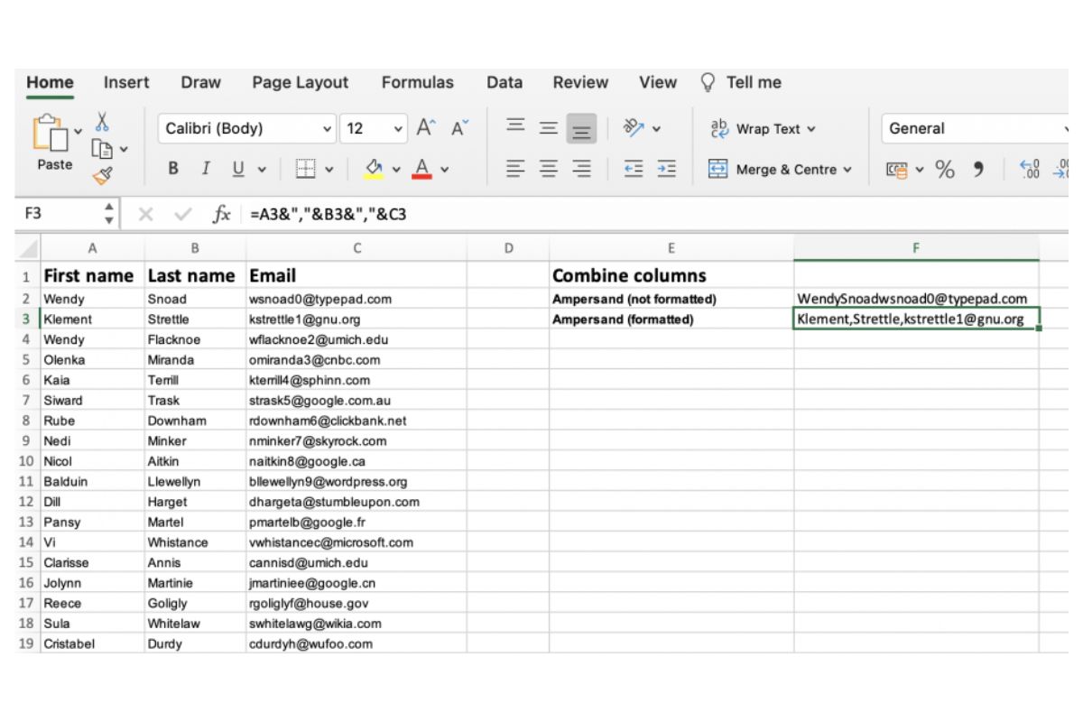
Another method to combine text with spaces or characters is to use the ampersand (&) operator. The ampersand allows you to concatenate text with ease. For instance, to merge the content of two columns with a space in between, you can use the following formula:
=A1 & " " & B1
This will join the text from cells A1 and B1, separated by a space.
By using these methods, you can combine text from different columns and insert custom characters or spaces to enhance the readability and structure of the merged data.
Combining Date and Time Columns
In Excel, combining date and time information from separate columns can be useful for performing calculations, creating reports, or analyzing data that includes both components. There are a few approaches to accomplish this.
One method is to use the CONCATENATE function along with the TEXT function to format the date and time values before combining them. For example, let’s say you have a date in column A (formatted as “mm/dd/yyyy”) and a time in column B (formatted as “hh:mm”). You can use the following formula to combine them:
=CONCATENATE(TEXT(A1, "mm/dd/yyyy"), " ", TEXT(B1, "hh:mm"))
This formula will format the date and time values using the TEXT function and then join them with a space in between.
An alternative approach is to use the ampersand (&) operator to concatenate the date and time values directly. Using the same example, the formula would be:
=TEXT(A1, "mm/dd/yyyy") & " " & TEXT(B1, "hh:mm")
By using the & operator, you can directly concatenate the formatted date and time values without the need for the CONCATENATE function.
It’s important to ensure that the date and time columns in Excel are recognized as valid dates and times. You can check this by verifying that the cells containing the dates and times are formatted as date or time values rather than plain text.
By combining date and time columns, you can create a unified timestamp that can be used for various calculations or analysis. This enables you to work with both components simultaneously and gain deeper insights from your data.
Combining Columns with Conditional Statements
Combining columns in Excel becomes more powerful when you can incorporate conditional statements to determine which values to include. This allows you to selectively merge data based on specific criteria or conditions.
One way to combine columns with conditional statements is to use the IF function. The IF function evaluates a logical condition and returns different values based on the outcome. You can include the IF function within the CONCATENATE or TEXTJOIN functions to control which values are merged.
For example, let’s say you have two columns in Excel: Column A contains a list of names, and Column B contains their corresponding ages. You might want to only combine the names of people who are above a certain age. You can use the following formula:
=IF(B1 > 18, A1, "")
This formula uses the IF function to check if the age in cell B1 is greater than 18. If it is, it includes the name from cell A1; otherwise, it returns an empty string (“”).
You can then use the CONCATENATE or TEXTJOIN function to merge the filtered names into a single column:
=CONCATENATE(IF(B1 > 18, A1, ""), ", ")
or
=TEXTJOIN(", ", TRUE, IF(B1 > 18, A1, ""))
These formulas will combine the names of people who are above 18 years old, with each name separated by a comma and a space.
By incorporating conditional statements into your column merging process, you have greater control over the data that gets combined. You can filter and include only the values that meet specific criteria, resulting in a more refined and meaningful output.
Handling Empty Cells and Errors While Combining Columns
When combining columns in Excel, you may come across situations where some cells are empty or contain errors. It is important to handle these scenarios properly to ensure accurate and error-free results in the merged column.
One approach to handle empty cells is to use an IF statement to check if a cell is empty before combining its value with other cells. For example, let’s say you have two columns in Excel: Column A contains text values, and Column B contains numbers. You want to merge these columns while ignoring any empty cells in either column. You can use the following formula:
=IF(OR(ISBLANK(A1), ISBLANK(B1)), "", CONCATENATE(A1, B1))
This formula checks if either cell A1 or B1 is empty using the ISBLANK function. If either cell is empty, it returns an empty string (“”). Otherwise, it combines the values using the CONCATENATE function.
In addition to empty cells, you may also encounter errors in the columns being merged. To handle errors, you can incorporate the IFERROR function into your formula. The IFERROR function allows you to replace error values with a specified value or action. For example, if you want to merge two columns and handle any errors gracefully, you can use the following formula:
=IFERROR(CONCATENATE(A1, B1), "Error!")
This formula attempts to combine the values from cells A1 and B1 using the CONCATENATE function. If an error occurs, such as a #VALUE! error, it replaces the error with the specified text string “Error!”.
By handling empty cells and errors properly while combining columns, you can ensure the accuracy and reliability of the merged data. It allows you to have control over what values are included and how errors are handled during the combination process.
Combining Columns with Line Breaks
Combining columns in Excel with line breaks can be useful when you want to merge data into a single cell while maintaining separate lines for each value. This is especially handy for generating address lists, multiline notes, or any other content where line breaks are important.
One method to achieve this is by using the CONCATENATE function along with the CHAR(10) function. The CHAR(10) function generates a line break or newline character within the formula.
For example, let’s say you have three columns in Excel: Column A contains street addresses, Column B contains city names, and Column C contains postal codes. You can use the following formula to merge these columns into a single cell with line breaks:
=CONCATENATE(A1, CHAR(10), B1, CHAR(10), C1)
This formula combines the text from cells A1, B1, and C1 and inserts a line break between each value using the CHAR(10) function. The result will be a multiline address with each component on a separate line.
An alternative approach is to use the ampersand (&) operator along with the TEXT function to format the line breaks. Using the same example, the formula would be:
=A1 & TEXT(10, "&")+ B1 & TEXT(10, "&") + C1
In this formula, the TEXT function is used to represent the line break within the concatenation string.
Once you have combined the columns with line breaks, be sure to format the cell to wrap text so that the lines are visible. You can do this by selecting the cell, navigating to the Home tab, and clicking the Wrap Text button in the Alignment group.
By combining columns with line breaks, you can create organized and visually appealing multiline content within a single cell. This helps to maintain the structure and readability of the merged data, particularly when dealing with address lists, notes, or other multiline information.
Combining Columns Using Formulas with Operators
In Excel, you can combine columns using formulas that incorporate operators to perform calculations or apply specific operations. This allows you to create advanced merged columns that include mathematical operations or manipulate the data in specific ways.
One common operator used for combining columns is the addition (+) operator. This operator allows you to sum numerical values from different columns. For example, if you have two columns in Excel, Column A contains numbers, and Column B contains numbers as well, you can use the following formula to add the values from both columns:
=A1 + B1
This formula will sum the values in cells A1 and B1 and give you the result in the merged cell.
Similarly, you can use other mathematical operators like subtraction (-), multiplication (*), and division (/) to perform calculations while combining columns. For instance, to multiply the values in Column A by the values in Column B, you can use the following formula:
=A1 * B1
The formula will multiply the values in cells A1 and B1 and provide the result in the merged cell.
Furthermore, you can also use comparison operators like greater than (>), less than (<), or equal to (=) to perform logical operations while combining columns. This enables you to include conditional statements within your formula. For example, if you have two columns of values and you only want to merge data when one column is greater than the other, you can use the following formula:
=IF(A1 > B1, A1, "")
This formula will check if the value in cell A1 is greater than the value in cell B1. If it is, it includes the value from cell A1 in the merged cell; otherwise, it returns an empty string.
By incorporating operators into your formulas while combining columns, you can perform calculations, apply mathematical operations, or implement logical conditions to manipulate the data and create more advanced merged columns in Excel.
Combining Columns without Formulas using Flash Fill
Excel provides a dynamic feature called Flash Fill that allows you to combine columns without the need for complex formulas. Flash Fill automatically recognizes patterns in your data and fills in the merged values for you.
To use Flash Fill, follow these simple steps:
- Start by typing the desired merged value in the first cell of the destination column.
- Press Enter to move to the next cell.
- On the Home tab, in the Editing group, click on the Flash Fill button, or press Ctrl + E.
- Excel will automatically detect the pattern and fill in the merged values for the remaining cells in the column.
For example, suppose you have two columns in Excel: Column A contains first names, and Column B contains last names. To combine these columns into a single column for the full name using Flash Fill, follow these steps:
- Type the full name in the first cell of the destination column, for example, “John Doe”.
- Press Enter, then navigate to the second cell in the destination column.
- Click the Flash Fill button or press Ctrl + E.
Excel will recognize the pattern and automatically fill in the merged values for the remaining cells with the full names.
Flash Fill can also handle more complex merging patterns. For instance, if you have a column with email addresses that follow a specific format, such as “firstname.lastname@example.com”, you can type one complete email address in the destination column and use Flash Fill to generate the merged values for the rest of the emails.
Flash Fill is a powerful tool that simplifies the process of combining columns in Excel without the need for formulas. It quickly recognizes patterns in your data and automates the merging process, saving you time and effort.