
What is the status bar in Excel?
The status bar is a useful feature in Microsoft Excel that provides quick and relevant information about the current status of your spreadsheet. It is located at the bottom of the Excel window and offers various tools and indicators that can assist you in your data analysis and spreadsheet management tasks.
One of the key functions of the status bar is to display the cell reference of the currently selected cell. This can be particularly helpful when working with large spreadsheets or when navigating through multiple sheets in a workbook. By glancing at the status bar, you can easily identify the row and column of the selected cell, allowing for quick and efficient data entry and editing.
In addition to the cell reference, the status bar also provides other essential information. For instance, it displays the sum, average, and count of selected cells with numerical values. This helps you obtain important statistical information without having to manually calculate it yourself. Furthermore, the status bar allows you to customize the displayed information, giving you the flexibility to choose the data that is most relevant to your current task.
Besides displaying data-related information, the status bar offers several useful tools. It includes a zoom slider that enables you to adjust the zoom level of your spreadsheet, making it easier to view and manage your data. The status bar also provides a page layout view button, allowing you to quickly switch between different views to see how your printed worksheet will look.
Furthermore, the status bar includes the fill handle, a convenient tool for quickly filling cells with data. By selecting a range of cells and dragging the fill handle, Excel can automatically fill in a series, such as dates or numbers, based on the pattern of the selected data.
Overall, the status bar in Excel is a valuable tool that provides essential information and useful features to enhance your productivity and simplify your data analysis tasks. Whether you need to quickly check the cell reference, perform basic calculations, adjust the zoom level, or use the fill handle to streamline your data entry, the status bar is there to assist you every step of the way.
How to display or hide the status bar in Excel
The status bar provides valuable information and tools in Excel, but there may be occasions when you want to toggle its visibility. Thankfully, Excel offers a simple way to display or hide the status bar based on your preference. Here’s how you can do it:
To display the status bar:
- Open Excel and navigate to the worksheet where you want to show the status bar.
- Go to the “View” tab in the Excel ribbon at the top of the window.
- In the “Show” group, make sure the “Status Bar” option is checked. If it’s already checked, then the status bar is already visible.
By following these steps, you can easily show the status bar in Excel, giving you access to its various functions and information.
To hide the status bar:
- Open Excel and go to the worksheet where you want to hide the status bar.
- Navigate to the “View” tab in the Excel ribbon at the top of the window.
- In the “Show” group, uncheck the “Status Bar” option. This will remove the status bar from the Excel window.
By following these steps, you can hide the status bar in Excel, allowing for a larger workspace or a cleaner view of your worksheet.
It’s important to note that when you hide the status bar, you won’t have access to the tools and information it provides. However, you can always toggle its visibility back on if needed.
Displaying or hiding the status bar in Excel gives you the flexibility to tailor your workspace to your specific needs. Whether you prefer the added functionality and information provided by the status bar or want a more streamlined view, Excel makes it easy to personalize your experience.
Overview of the different elements in the status bar
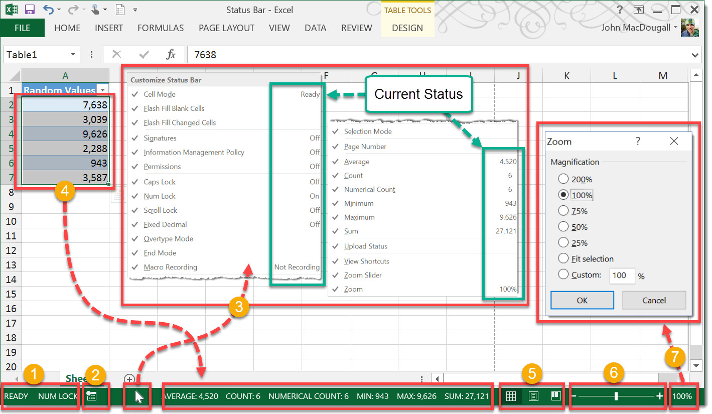
The status bar in Excel consists of several elements that provide valuable information and quick access to essential tools. Understanding these elements can help you make the most of this feature. Here is an overview of the different elements in the status bar:
1. Cell Reference: This element displays the current cell reference, showing the column letter and the row number of the selected cell. It helps you keep track of your position within the spreadsheet and facilitates data entry and editing.
2. Sum, Average, Count: These functions are located on the right side of the status bar. When you select a range of cells with numerical values, Excel automatically calculates and displays the sum, average, and count of those values. This allows you to quickly analyze and interpret your data without the need for manual calculations.
3. Zoom Slider: The zoom slider appears as a percentage on the right side of the status bar. It enables you to adjust the magnification level of your spreadsheet, making it easier to view and work with your data. Simply drag the slider to the desired zoom level or use the increase and decrease buttons to fine-tune the zoom.
4. Page Layout View Button: This button, located next to the zoom slider, provides quick access to the page layout view. Clicking on it allows you to see how your printed worksheet will look, making it easier to adjust margins, headers, footers, and other page settings.
5. Fill Handle: The fill handle is a small square located at the lower-right corner of the selected cell or range. It is used for quick data entry and allows you to automatically fill cells with a series of data based on a pattern. By dragging the fill handle, you can extend and complete a series, such as dates, numbers, or text.
6. Customization Options: The status bar can be customized to display additional information depending on your needs. You can right-click on the status bar to access a menu that allows you to enable or disable various options, such as displaying the average, minimum, maximum, or numerical count of the selected range.
By becoming familiar with the different elements in the status bar, you can efficiently utilize its functions and data analysis capabilities. From quickly accessing cell references and performing calculations to adjusting zoom levels and utilizing the fill handle, the status bar offers a range of features that can enhance your Excel experience.
Using the zoom slider in the status bar
The zoom slider in the status bar of Excel is a powerful tool that allows you to adjust the magnification level of your spreadsheet. With the zoom slider, you can easily increase or decrease the size of the cells and text, making it easier to view and work with your data. Here’s how you can utilize the zoom slider:
1. Locate the Zoom Slider: The zoom slider is located on the right side of the status bar, next to the percentage display. It is represented by a slider with a plus (+) and minus (-) sign.
2. Adjust the Zoom Level: To zoom in, click on the plus sign (+) or drag the slider to the right. This will increase the magnification level, making the cells and text larger. To zoom out, click on the minus sign (-) or drag the slider to the left. This will decrease the magnification level, making the cells and text smaller.
3. Use the Increase and Decrease Buttons: Alternatively, you can use the increase and decrease buttons located on the right side of the slider. Each click on the increase button will increment the zoom level by 10%, and each click on the decrease button will decrement it by 10%.
4. Customize the Zoom Level: If you need a specific zoom level that is not available on the slider, you can click on the zoom percentage display next to the slider. This will open the zoom dialog box, where you can specify a custom zoom percentage or select from predefined options.
5. Fit to Window: To quickly fit the entire spreadsheet within the current Excel window, double-click on the zoom percentage display. Excel will automatically adjust the zoom level so that all the content is visible without any horizontal or vertical scrolling.
By using the zoom slider in the status bar, you can easily adapt the view of your spreadsheet to your specific needs. Whether you need a closer look at the details or a broader overview of your data, the zoom slider provides the flexibility to adjust the magnification level quickly and effortlessly.
Using the page layout view in the status bar
The page layout view is a useful feature in Excel that allows you to see how your printed worksheet will look. The page layout view provides a more accurate representation of your data, including headers, footers, margins, and other page settings. This view is easily accessible through the status bar in Excel. Here’s how you can make use of the page layout view:
1. Locate the Page Layout View Button: The page layout view button is located on the right side of the status bar, next to the zoom slider and percentage display. The button looks like a small page with lines on it.
2. Click on the Page Layout View Button: To enter the page layout view, simply click on the page layout view button in the status bar. This will switch your current view to the page layout view, providing a realistic representation of your worksheet as it would appear when printed.
3. Adjust Page Layout Settings: While in the page layout view, you can modify various page layout settings to ensure your worksheet looks exactly how you want it to. You can adjust margins, headers and footers, orientation (portrait or landscape), and page breaks, among other options. Simply navigate to the “Page Layout” tab in the Excel ribbon to access these settings.
4. Edit Cells and Data in Page Layout View: Even in the page layout view, you can still edit cells and data as you would in other Excel views. Simply click on a cell and start typing or make changes as needed. The page layout view provides a convenient combination of the realistic page representation and the ability to edit your data.
5. Switch Back to Normal View: Once you have finished making adjustments or reviewing your worksheet in the page layout view, you can switch back to the normal view by either clicking on the “Normal” view button at the bottom-right corner of the Excel window or by clicking on the page layout view button again in the status bar.
By using the page layout view in the status bar, you can ensure that your worksheet is visually appealing and formatted correctly for printing. This view provides a helpful way to preview and adjust your page layout settings before printing, saving you time and effort in the printing process.
Using the fill handle in the status bar
The fill handle in the status bar of Excel is a convenient tool that allows you to quickly fill cells with data based on a pattern. It can save you time and effort when populating a series of data, such as dates, numbers, or text. Here’s how you can make use of the fill handle:
1. Select the Initial Cell: Start by selecting the cell or range that contains the initial value or pattern that you want to fill. When you hover over the bottom-right corner of the selected cell, the fill handle will appear as a small square.
2. Drag the Fill Handle: Click and hold the fill handle, then drag it in the desired direction. Excel will automatically fill in the cells in the selected range based on the pattern of the initial value or series. The cells will be populated with values that follow the same pattern, continuing the series or filling in the appropriate data.
3. Options for Filling: When you drag the fill handle, Excel offers several options for filling depending on the content of the initial cell. For example, if the initial cell contains a numerical series, Excel will continue the series by incrementing the values as you drag the fill handle. If the initial cell contains a date or day of the week, Excel will generate the next dates or days accordingly.
4. Extending the Fill Series: If you want to extend the fill series beyond the initial range, simply continue dragging the fill handle in the desired direction. Excel will automatically adjust the values based on the pattern to fill in the additional cells.
5. Additional Fill Options: Right-clicking on the fill handle opens a context menu with additional fill options. For example, you can choose to fill only the formatting or fill series without formatting. This gives you more control over how the data is populated in the selected range.
By utilizing the fill handle, you can significantly speed up the process of filling cells with a series, saving you time and effort in data entry. Whether you need to populate cells with dates, numbers, or text, the fill handle in the status bar provides a simple and efficient solution.
Using the sum function in the status bar
The sum function in the status bar of Excel is a handy tool that allows you to quickly calculate the sum of selected cells containing numerical values. It eliminates the need for manual calculations and provides instant results, saving you time and effort. Here’s how you can make use of the sum function:
1. Select the Cells: Start by selecting the range of cells that you want to calculate the sum for. Ensure that the cells contain numerical values that you want to include in the sum calculation.
2. Locate the Sum Display: Once you have selected the cells, look for the sum display located in the status bar at the bottom of the Excel window. It will show the sum of the numbers in the selected range.
3. View the Sum: The sum in the status bar updates automatically as you select different cells or change the values in the selected range. It provides you with a dynamic and real-time calculation of the sum of the selected cells.
4. Customize the Sum Display: By default, the sum display in the status bar shows the sum of the selected range. However, you can customize it to show other statistics, such as average, count, or numerical count, by right-clicking on the status bar and selecting the desired option.
5. Additional Sum Options: Right-clicking on the sum display in the status bar opens a context menu with additional options. For example, you can choose to display the sum as a percentage of the total or exclude hidden cells from the sum calculation. These options provide added flexibility and control over the sum function.
By utilizing the sum function in the status bar, you can easily calculate the sum of selected cells without the need for complex formulas or manual calculations. Whether you’re working with a small range or a large dataset, the sum function simplifies data analysis and enhances your efficiency in Excel.
Using the average function in the status bar
The average function in the status bar of Excel is a valuable tool that allows you to quickly calculate the average of selected cells containing numerical values. It saves you time and effort by providing instant results without the need for manual calculations. Here’s how you can make use of the average function:
1. Select the Cells: Start by selecting the range of cells that you want to calculate the average for. Ensure that the cells contain numerical values that you want to include in the average calculation.
2. Locate the Average Display: Once you have selected the cells, look for the average display located in the status bar at the bottom of the Excel window. It will show the average of the numbers in the selected range.
3. View the Average: The average in the status bar updates automatically as you select different cells or change the values in the selected range. It provides you with a dynamic and real-time calculation of the average of the selected cells.
4. Customize the Average Display: By default, the average display in the status bar shows the average of the selected range. However, you can customize it to show other statistics, such as sum, count, or numerical count, by right-clicking on the status bar and selecting the desired option.
5. Additional Average Options: Right-clicking on the average display in the status bar opens a context menu with additional options. For example, you can choose to display the average as a percentage of the total or exclude hidden cells from the average calculation. These options provide added flexibility and control over the average function.
By utilizing the average function in the status bar, you can easily calculate the average of selected cells without the need for complex formulas or manual calculations. Whether you’re working with a small range or a large dataset, the average function simplifies data analysis and enhances your efficiency in Excel.
Using the count function in the status bar
The count function in the status bar of Excel is a powerful tool that allows you to quickly determine the number of selected cells containing numerical values. It eliminates the need for manual counting and provides instant results, saving you time and effort. Here’s how you can make use of the count function:
1. Select the Cells: Start by selecting the range of cells that you want to count. Ensure that the cells contain the values that you want to include in the count calculation.
2. Locate the Count Display: Once you have selected the cells, look for the count display located in the status bar at the bottom of the Excel window. It will show the count of the cells in the selected range that contain numerical values.
3. View the Count: The count in the status bar updates automatically as you select different cells or change the values in the selected range. It provides you with a dynamic and real-time calculation of the number of cells that contain numerical values.
4. Customize the Count Display: By default, the count display in the status bar shows the count of the selected cells that contain numerical values. However, you can customize it to show other statistics, such as sum, average, or numerical count, by right-clicking on the status bar and selecting the desired option.
5. Additional Count Options: Right-clicking on the count display in the status bar opens a context menu with additional options. For example, you can choose to display the count as a percentage of the total or exclude hidden cells from the count calculation. These options provide added flexibility and control over the count function.
By utilizing the count function in the status bar, you can easily determine the number of selected cells containing numerical values without the need for manual counting or complex formulas. Whether you’re working with a small range or a large dataset, the count function simplifies data analysis and enhances your efficiency in Excel.
Using the numerical count function in the status bar
The numerical count function in the status bar of Excel is a useful tool that allows you to quickly determine the number of selected cells containing numerical values. It provides an instant count without including empty cells or cells with non-numerical data, saving you time and effort. Here’s how you can make use of the numerical count function:
1. Select the Cells: Start by selecting the range of cells that you want to count. Ensure that the cells contain the values that you want to include in the numerical count calculation.
2. Locate the Numerical Count Display: Once you have selected the cells, look for the numerical count display located in the status bar at the bottom of the Excel window. It will show the count of the cells in the selected range that contain numerical values.
3. View the Numerical Count: The numerical count in the status bar updates automatically as you select different cells or change the values in the selected range. It provides you with a dynamic and real-time calculation of the number of cells that contain numerical values.
4. Customize the Numerical Count Display: By default, the numerical count display in the status bar shows the count of the selected cells that contain numerical values. However, you can customize it to show other statistics, such as sum, average, or count, by right-clicking on the status bar and selecting the desired option.
5. Additional Numerical Count Options: Right-clicking on the numerical count display in the status bar opens a context menu with additional options. For example, you can choose to display the numerical count as a percentage of the total or exclude hidden cells from the count calculation. These options provide added flexibility and control over the numerical count function.
By utilizing the numerical count function in the status bar, you can easily determine the number of selected cells containing numerical values without including empty cells or cells with non-numerical data. It simplifies data analysis and enhances your efficiency, particularly when working with large datasets or when accuracy is crucial.
How to customize the status bar in Excel
The status bar in Excel can be customized to display different types of information based on your specific needs. By customizing the status bar, you can choose to show or hide various options and statistics to enhance your data analysis and workflow. Here’s how you can customize the status bar in Excel:
1. Right-click on the Status Bar: To access the customization options for the status bar, simply right-click anywhere on the status bar itself. A context menu will appear with a list of available options.
2. Select the Options: In the context menu, you will see a list of options that you can enable or disable. The options include displaying the average, count, numerical count, minimum, maximum, and more. Simply click on the option you want to enable or disable to customize the status bar to your preference.
3. Customize the Summary Calculation: In addition to displaying single statistics, you can also customize the summary calculation shown in the status bar. For example, you can change the calculation from the default “Sum” to “Average” or “Count” by right-clicking on the sum display and selecting the desired calculation method.
4. Additional Customization Options: Excel also offers additional customization options for the status bar. By going to the “Options” menu, accessible from the Excel main menu, you can access advanced settings. Here, you can choose to customize the display of the status bar based on specific preferences, such as excluding hidden cells or showing the percentage of the total.
5. Save and Apply Changes: Once you have finished customizing the status bar, your changes will be applied immediately. The status bar will now display the information and statistics based on your customization selections.
By customizing the status bar in Excel, you can tailor it to display the information that is most relevant to your work. Whether you want to focus on specific calculations, get a quick overview of your data, or hide certain information to simplify the view, the status bar customization options give you the flexibility to adapt it to your specific needs.
Additional tips and tricks for using the status bar in Excel
The status bar in Excel offers more than just displaying information and providing quick access to tools. There are several additional tips and tricks that can further enhance your efficiency and productivity when using the status bar. Here are some valuable tips to consider:
1. Utilize keyboard shortcuts: To quickly access frequently used functions in the status bar, you can use keyboard shortcuts. For example, you can press Alt and the corresponding number key to toggle specific summary calculations directly. Alt+1 will toggle sum, Alt+2 for average, Alt+3 for count, and so on.
2. Take advantage of tooltips: When you hover over certain elements in the status bar, tooltips will appear to provide additional information. These tooltips can offer useful insights and explanations, helping you better understand and utilize the various features and functions available.
3. Show more summary calculations: By default, the status bar displays the sum, average, and count. However, you can right-click on the status bar to access the customization options and enable additional summary calculations, such as minimum, maximum, and numerical count. This allows you to have a comprehensive overview of your data without needing to perform manual calculations.
4. Use the status bar as a quick data entry tool: The status bar also acts as a convenient data entry tool. With multiple cells selected, the status bar can show the sum, average, or count of the selected cells, allowing you to quickly input these values into another cell without needing to use functions or formulas.
5. Detect errors: In addition to providing calculations and information, the status bar can show error indicators when certain errors are detected in your worksheet. Whether it’s a #DIV/0! error or a circular reference warning, the status bar can alert you to potential issues that need attention.
6. Resize the status bar: If the default size of the status bar is not optimal for your workspace, you can resize it by clicking and dragging the border of the status bar. Adjusting the size allows you to show more or fewer elements depending on your preference and screen real estate.
By utilizing these additional tips and tricks, you can make the most out of the status bar in Excel. Whether it’s customizing the display, using keyboard shortcuts, taking advantage of tooltips, or using the status bar as a quick data entry tool, these techniques can enhance your productivity and streamline your workflows in Excel.