
What is the AVERAGEIF function?
The AVERAGEIF function is a powerful tool in Excel that allows you to calculate the average of a range of numbers based on specific criteria. It is particularly useful when you want to find the average of a subset of data that meets certain conditions.
With the AVERAGEIF function, you can specify a range of values to evaluate and a criterion to determine which values should be included in the average calculation. This criterion can be a number, a cell reference, a text string, or a logical expression.
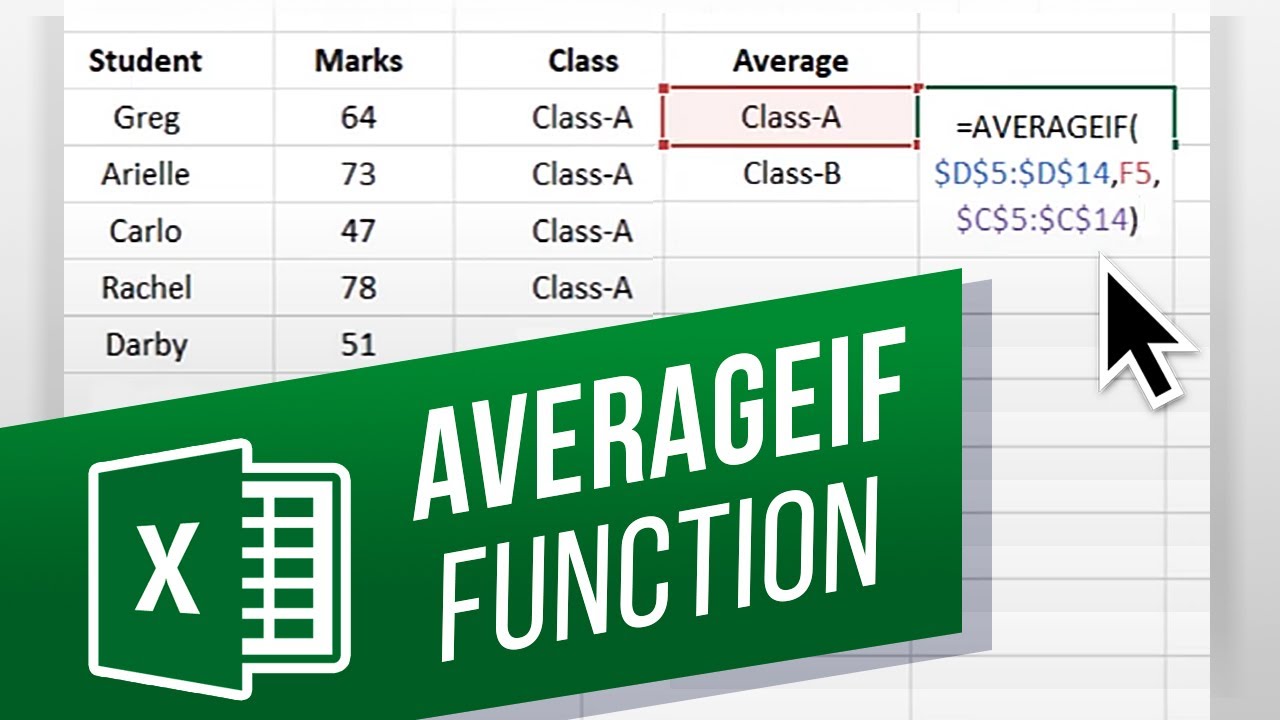
The AVERAGEIF function follows a simple syntax:
=AVERAGEIF(range, criteria, [average_range])
The range argument refers to the range of values to be evaluated, while the criteria argument specifies the conditions that must be met for a value to be included in the average calculation.
The optional average_range argument defines the range of values to be averaged. If this argument is omitted, the AVERAGEIF function will use the range argument as the average range.
The AVERAGEIF function is highly versatile and can be used in various scenarios. It allows you to easily filter and calculate averages based on specified criteria without the need for complex formulas or manual filtering.
Now that we understand the basics of the AVERAGEIF function, let’s explore how to use it to tackle the problem of ignoring zeros in averages.
How to Use the AVERAGEIF Function
Using the AVERAGEIF function in Excel is straightforward and requires a few simple steps. Here’s how you can utilize this function to calculate averages based on specific criteria:
Step 1: Set up your data
First, ensure that your data is organized in columns or rows. For example, you might have a column of values representing sales figures for different products, and you want to calculate the average sales for a certain category.
Step 2: Use the AVERAGEIF function to calculate the average
Next, select a cell where you want to display the calculated average. Enter the formula =AVERAGEIF(range, criteria) in the cell, replacing range with the range of values you want to evaluate and criteria with the conditions that determine which values to include in the average calculation.
Step 3: Add the criteria to ignore zeros
If you want to exclude zero values from the average calculation, you can add an additional criterion using the “not equal to” operator (<>). For example, to ignore zeros in the average sales calculation, you would modify the formula to =AVERAGEIF(range, "<>0").
Step 4: Complete the formula and get the desired average
Press Enter to calculate the average based on the specified criteria. The cell will now display the average value.
The AVERAGEIF function will evaluate the range of values and include only those that meet the specified criteria. It will then calculate the average of the selected values.
Remember, the AVERAGEIF function allows for flexible criteria. You can use comparison operators, such as greater than (>) or less than (<), and combine multiple criteria using logical operators like AND or OR to get precise average calculations.
Now that you know how to use the AVERAGEIF function, let’s dive into the solution to ignoring zeros in averages.
The Problem with Zeros in Averages
When calculating averages in Excel, including zero values can sometimes skew the results and provide inaccurate insights. Zeros can significantly impact the average, especially if they are not representative of the data you’re analyzing. This can be problematic if you want to focus on non-zero values or exclude outliers from your calculations.
For example, consider a dataset representing monthly sales for a product. If you include zero sales in the average, it may artificially lower the average and not accurately reflect the performance of the product. Ignoring zeros can provide a more realistic average that aligns with your intended analysis.
Furthermore, when working with large datasets or complex calculations, including zero values can make it more difficult to identify trends or patterns. By excluding zeros from your averages, you can emphasize the data points that are more relevant and meaningful to your analysis.
However, Excel’s default average calculations consider all values, including zeros. This poses a challenge when you specifically want to ignore zeros while calculating averages.
Fortunately, Excel provides a solution for this problem—the AVERAGEIF function, which allows you to set criteria to selectively include or exclude values from the average calculation. By leveraging the AVERAGEIF function, you can easily overcome the issue of including zeros and obtain more accurate averages that better represent your data.
Now that we understand the problem with zeros in averages, let’s explore how the AVERAGEIF function can be used to ignore zeros and calculate more precise averages.
The Solution: Ignore Zeros with the AVERAGEIF Function
To address the problem of including zeros in averages, Excel provides the AVERAGEIF function, which allows you to specify criteria to selectively include or exclude values from the average calculation. By utilizing this function, you can easily ignore zeros and obtain more accurate average values.
Step 1: Set up your data
Before using the AVERAGEIF function, ensure that your data is structured in columns or rows. This could be a range of values representing sales figures, test scores, or any other set of numerical data.
Step 2: Use the AVERAGEIF function to calculate the average
Select a cell where you want the average to be displayed, and input the formula =AVERAGEIF(range, criteria). Replace range with the range of values you wish to evaluate, and criteria with the conditions for selecting values for the average calculation.
Step 3: Add the criteria to ignore zeros
To exclude zero values from the average calculation, add an additional criterion using the “not equal to” operator, <>. For example, you can modify the formula to =AVERAGEIF(range, "<>0").
Step 4: Complete the formula and obtain the desired average
Press Enter to calculate the average, and the cell will display the resulting value. The AVERAGEIF function will evaluate the specified range of values and include only those that meet the criteria, ignoring any zeros.
By using the AVERAGEIF function with the criteria "<>0", zero values will be excluded from the average calculation. This allows you to focus solely on the non-zero values, providing a more meaningful and accurate representation of the data.
Remember, the AVERAGEIF function offers flexibility in defining criteria. You can use comparison operators, such as greater than or less than, and combine multiple conditions if necessary to precisely calculate the average.
Now that we have explored the solution of ignoring zeros with the AVERAGEIF function, let’s move on to the practical steps of using this function to obtain reliable averages.
Step 1: Set up your data
Before you can use the AVERAGEIF function to calculate averages and ignore zeros in Excel, it’s essential to ensure that your data is properly set up. By organizing your data in a structured manner, you will enable the AVERAGEIF function to accurately evaluate and calculate the desired average based on specific criteria.
Here are some key considerations when setting up your data:
- Columns or rows: Decide whether to arrange your data vertically in columns or horizontally in rows. This will depend on the nature of your data and how you want to analyze it. Ensure that the range of values you want to evaluate is within a single column or row.
- Data range: Determine the range of values that you want to include in the average calculation. This could be a range of numbers representing prices, quantities, or any other relevant data points.
- Categorical data: If you have categorical data that you want to use as criteria in the AVERAGEIF function, ensure that the categories are properly labeled and organized.
By structuring your data, you will make it easier to specify the range and criteria in the AVERAGEIF function, allowing Excel to accurately calculate the desired average.
For example, imagine you have a dataset of sales for different products over several months. In this case, you might structure your data with each product in a column and the monthly sales figures in rows. This arrangement will enable you to easily select the range of values you want to evaluate when using the AVERAGEIF function.
Before moving on to the next step, take the time to ensure that your data is well-organized and aligned with the objectives of your average calculation. By doing so, you will set a solid foundation for utilizing the AVERAGEIF function and obtaining accurate averages in Excel.
Step 2: Use the AVERAGEIF function to calculate the average
Once you have your data properly set up, you can now proceed to use the AVERAGEIF function in Excel to calculate the average based on specific criteria. The AVERAGEIF function allows you to selectively include or exclude values from the average calculation, providing a powerful tool for tailored data analysis.
Here’s how you can use the AVERAGEIF function to calculate the average:
- Select the cell where you want to display the calculated average.
- Enter the formula
=AVERAGEIF(range, criteria)into the cell. - Replace
rangewith the range of values you want to evaluate for the average calculation. - Provide a criterion in the
criteriaargument that specifies the conditions for including values in the average calculation.
For example, suppose you have a column of sales figures for different products, and you want to calculate the average sales for a specific category. You would select a cell where you want the result to appear, enter the formula =AVERAGEIF(range, category), and replace range with the range of sales figures and category with the specific category you want to evaluate.
The AVERAGEIF function will then evaluate the range of values and calculate the average based on the specified criterion. The resulting value will be displayed in the cell you selected.
Using the AVERAGEIF function simplifies the process of calculating averages based on specific criteria. Instead of manually filtering data or applying complex formulas, you can easily specify the range and criterion within the function to obtain the desired average.
Now that you know how to use the AVERAGEIF function to calculate averages, let’s move on to the third step, where we’ll learn how to add criteria to ignore zeros in the average calculation.
Step 3: Add the Criteria to Ignore Zeros
By default, the AVERAGEIF function considers all values within the specified range when calculating the average. If you want to exclude zero values from the average calculation, you can add an additional criterion that instructs Excel to ignore zeros.
Here’s how you can add the criteria to ignore zeros in the AVERAGEIF function:
- Open the cell where you’ve entered the AVERAGEIF formula.
- Modify the formula to include the criterion
"<>0"within thecriteriaargument. This criterion states that the value should be “not equal to” zero.
For instance, if you want to calculate the average of sales figures but exclude zero sales, you would modify the formula to =AVERAGEIF(range, "<>0"). The “<>” symbol represents “not equal to” in Excel. This additional criterion ensures that any zero values within the specified range are not included in the average calculation.
By adding this criteria, Excel will consider only the values that meet the specified conditions for the average calculation. Zero values will be ignored, providing you with a more accurate average that reflects the data points you want to focus on.
It’s essential to carefully consider the criteria you specify to ensure it accurately reflects the data you want to include or exclude from the average calculation. You can use other comparison operators like “<“, “>“, “<=“, or “>=” in combination with the “<>” operator to set more specific criteria for filtering the values.
With the added criteria to ignore zeros, the AVERAGEIF function becomes a valuable tool for obtaining precise averages that align with your analysis goals.
Now that you’ve learned how to add the criteria to ignore zeros, let’s move on to the final step, where we’ll complete the formula and obtain the desired average.
Step 4: Complete the Formula and Get the Desired Average
After adding the criteria to ignore zeros in the AVERAGEIF function, you’re now ready to complete the formula and obtain the desired average. With this final step, you’ll calculate the average based on the specified range and criteria, ensuring that zero values are excluded from the calculation.
Here’s how you can complete the formula and obtain the desired average:
- Press Enter or click out of the cell that contains the AVERAGEIF formula.
- Excel will now calculate the average based on the defined range and criteria, and display the resulting average in the selected cell.
By completing the formula, Excel will evaluate the specified range of values, apply the criteria to exclude zeros, and calculate the average based on the remaining values.
For example, if you have a range of sales figures and you’ve added the criteria "<>0" to exclude zero sales, pressing Enter will trigger Excel to calculate the average sales based on the non-zero values. The resulting average will then be displayed in the cell where you entered the formula.
The completed formula allows you to obtain an accurate average that reflects the values you want to include in your analysis, while excluding any zeros that could skew the result.
Remember, the AVERAGEIF function is dynamic and will update automatically if you make changes to the range or criteria. This flexibility allows you to easily adapt your average calculations as your data evolves.
With the completion of the formula and the resulting average displayed, you have successfully used the AVERAGEIF function to calculate averages while ignoring zeros.
Now that you have completed all the steps, you can utilize the AVERAGEIF function to obtain meaningful and precise averages in Excel.
Additional Tips for Using AVERAGEIF with Ignored Zeros
While you now know how to use the AVERAGEIF function to calculate averages while ignoring zeros, there are a few additional tips that can further enhance your data analysis and optimize your use of this powerful function.
Here are some additional tips for using AVERAGEIF with ignored zeros:
- Combine criteria: You can use multiple criteria within the AVERAGEIF function to further refine your average calculation. By using logical operators like AND or OR, you can specify more complex conditions for including or excluding values. This allows you to create precise criteria that suit your analysis needs.
- Update criteria dynamically: If your criteria might change frequently, consider storing the criteria in separate cells. This way, you can easily modify the criteria without editing the formula directly. By referencing the criteria from cells, your average calculation will update dynamically whenever you change the criteria values.
- Highlight ignored zeros: To clearly visualize the exclusion of zeros from your average calculation, consider formatting the zero values with a different color. This makes it easier to identify which values are included or excluded from the calculation and provides a visual representation of the data selection process.
- Utilize wildcard characters: If you have text values in your range and want to exclude specific text patterns, you can use wildcard characters like asterisks (*) or question marks (?) in your criteria. This allows you to match and exclude text values based on certain patterns or conditions.
- Experiment with other functions: Excel offers various other functions, such as AVERAGEIFS and AGGREGATE, that provide more advanced functionalities for calculating averages based on specific criteria. These functions might be useful in scenarios where you need to incorporate multiple criteria or perform complex calculations.
By implementing these additional tips, you can improve the precision, flexibility, and efficiency of your average calculations with the AVERAGEIF function.
Remember to adapt these tips to your specific analysis requirements and explore the various possibilities that Excel offers. By leveraging the full potential of the AVERAGEIF function and other related functions, you can achieve accurate and insightful averages in your data analysis.