How to Remove Duplicates in Excel

Find Duplicates Using Conditional Formatting

Duplicates in Excel can make data analysis and manipulation more challenging. However, with the help of conditional formatting, you can easily spot and identify duplicate entries in your Excel spreadsheets. Conditional formatting is a powerful feature that allows you to apply specific formatting rules to cells based on their values or contents.

Here’s how you can find duplicates using conditional formatting:

Select the range of cells that you want to check for duplicates.
Navigate to the ‘Home’ tab in the Excel ribbon and click on ‘Conditional Formatting’ in the ‘Styles’ group.
From the dropdown menu, choose ‘Highlight Cells Rules’ and then select ‘Duplicate Values’.
In the ‘Duplicate Values’ dialog box, choose the formatting style you prefer for highlighting duplicates, such as bold or colored cells.
Click ‘OK’ to apply the conditional formatting to the selected range.

Once you have applied conditional formatting, any duplicate values within the selected range will be highlighted according to the formatting style you chose. This makes it easy to identify and analyze duplicate entries in your Excel spreadsheet.

It’s important to note that conditional formatting only highlights duplicates; it does not automatically remove them. To remove duplicates, you will need to use one of the methods mentioned in the following sections.

By utilizing the power of conditional formatting, you can effectively identify duplicate data in your Excel worksheets, making it easier to clean up and work with your data.

Remove Duplicates Using Excel’s Built-in Feature

Excel provides a convenient built-in feature that allows you to easily remove duplicate entries from your spreadsheets. This feature automatically analyzes the data in the selected range and removes any duplicate values, leaving only the unique values behind.

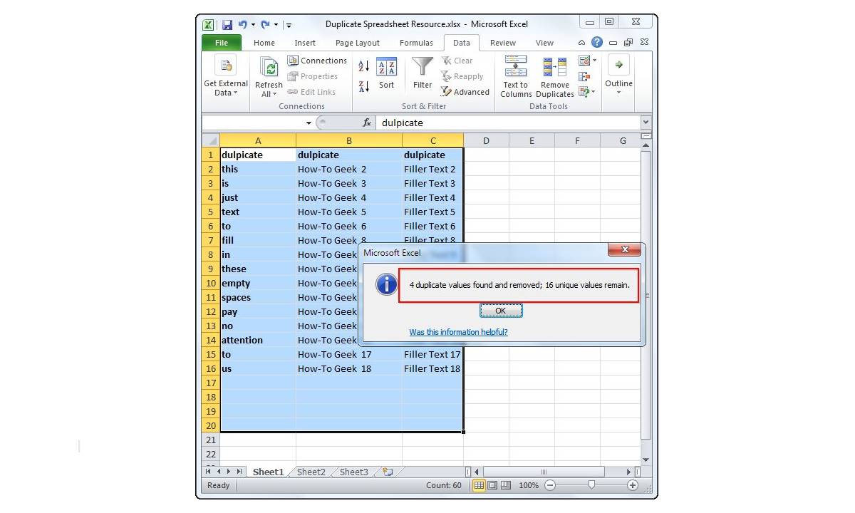
Here’s how you can remove duplicates using Excel’s built-in feature:

Select the range of cells that you want to remove duplicates from.
Navigate to the ‘Data’ tab in the Excel ribbon and click on ‘Remove Duplicates’ in the ‘Data Tools’ group.
In the ‘Remove Duplicates’ dialog box, choose the columns that you want to check for duplicates. By default, Excel checks for duplicates in all columns of the selected range.
Click ‘OK’ to remove duplicates and keep the first occurrence of each unique value.

Excel will automatically remove duplicate entries from the selected range, keeping only the first occurrence of each unique value. The remaining data will be rearranged to fill any gaps created by the removed duplicates.

Please note that this method permanently removes duplicates from the spreadsheet. It is advisable to make a backup of your data before using this feature.

By utilizing Excel’s built-in feature to remove duplicates, you can streamline your data and ensure that only unique values remain, making it easier to analyze and work with your spreadsheets.

Remove Duplicates Using Advanced Filters

If you prefer more control over the removal of duplicates in your Excel spreadsheet, you can use the Advanced Filters feature. This feature allows you to define specific criteria to filter and extract unique values from a dataset.

Here’s how you can remove duplicates using Advanced Filters:

Select the range of cells that you want to remove duplicates from.
Navigate to the ‘Data’ tab in the Excel ribbon and click on ‘Advanced’ in the ‘Sort & Filter’ group.
In the ‘Advanced Filter’ dialog box, choose the ‘Copy to another location’ option.
In the ‘Copy to’ field, specify the range where you want to copy the unique values.
Check the ‘Unique records only’ box to filter out duplicates.
Click ‘OK’ to apply the advanced filter and copy the unique values to the specified location.

Excel will analyze the selected range and copy only the unique values, based on the criteria you provided, to the specified location. This method allows you to keep the original dataset intact and have more control over the filtering process.

It’s important to note that if you have multiple columns in your dataset, the Advanced Filters feature will remove duplicates based on the values in all selected columns.

By using the Advanced Filters feature in Excel, you can precisely remove duplicates from your dataset while preserving the flexibility to define specific filtering criteria for your unique values.

Remove Duplicates Using Formulas

If you want to remove duplicates in Excel while keeping the original dataset intact, you can utilize formulas to identify and eliminate duplicate entries. By using a combination of functions, you can create a formula that checks for duplicates and returns only the unique values.

Here’s how you can remove duplicates using formulas:

Create a new column next to the column that contains the data in which you want to remove duplicates.
In the first cell of the new column, enter the formula that checks for duplicates. For example, you can use the formula =COUNTIF($A$2:$A$10, A2) to check how many occurrences of the value in cell A2 exist in the range A2:A10.
Drag the formula down to apply it to the entire column.
In another column, enter the formula that extracts only the unique values. You can use the formula =IF(B2=1, A2, "") to display the value in cell A2 only if the corresponding count in column B is 1.
Drag the formula down to apply it to the entire column.
Select and copy the entire column containing the unique values.
Paste the values in a new location to separate them from the original dataset.

By using formulas, you can dynamically identify duplicates and extract only the unique values without altering the original data. This method allows you to have more control over the removal of duplicates and can be applied to multiple columns if needed.

Keep in mind that formulas may require additional adjustments based on your specific dataset and requirements. However, by utilizing formulas, you can effectively remove duplicates and retain the flexibility to customize the process according to your needs.

Remove Duplicates Using VBA Macro

If you frequently work with large datasets and need to remove duplicates in Excel, using a VBA macro can automate the process and save you time. VBA (Visual Basic for Applications) is a programming language that allows you to create custom macros and automate tasks in Excel.

Here’s how you can remove duplicates using a VBA macro:

Open the VBA Editor by pressing Alt + F11 in Excel.
In the VBA Editor, insert a new module by clicking on ‘Insert’ and selecting ‘Module’.
In the module, copy and paste the following VBA code:

vba
Sub RemoveDuplicates()
Dim rng As Range
Set rng = Selection

rng.RemoveDuplicates Columns:=Array(1), Header:=xlYes
End Sub

This simple VBA macro removes duplicates from the selected range and keeps the first occurrence of each unique value.

Press F5 to run the macro.

The macro will automatically remove duplicates from the selected range, leaving only the unique values behind. You can modify the code to customize the columns to check for duplicates or change the behavior of the removal process.

Using VBA macros can streamline and automate the removal of duplicates, especially when working with large datasets. With a little programming knowledge, you can create powerful macros that cater to your specific requirements.

Remove Duplicates Keeping the First Occurrence

When removing duplicates from your Excel spreadsheet, you may want to keep the first occurrence of each unique value while eliminating any subsequent duplicates. Excel provides built-in functionality that allows you to easily accomplish this task.

Here’s how you can remove duplicates while keeping the first occurrence:

Select the range of cells from which you want to remove duplicates.
Navigate to the ‘Data’ tab in the Excel ribbon and click on ‘Remove Duplicates’ in the ‘Data Tools’ group.
In the ‘Remove Duplicates’ dialog box, choose the columns that you want to check for duplicates. By default, Excel checks for duplicates in all columns of the selected range.
Uncheck all columns except the one that contains the data you want to keep the first occurrence of.
Click ‘OK’ to remove duplicates, ensuring that only the first occurrence of each unique value is retained.

Excel will analyze the selected range and remove any subsequent duplicates, keeping only the first occurrence of each unique value based on the column you specified. The remaining data will be rearranged to fill any gaps created by the removed duplicates.

By using this feature, you can efficiently eliminate duplicate values while preserving the original dataset and ensuring that the first occurrence of each unique value remains intact.

Remove Duplicates Keeping the Last Occurrence

If your Excel dataset contains duplicates and you want to keep the last occurrence of each unique value, there is a method within Excel’s built-in functionality that allows you to achieve this.

Here’s how you can remove duplicates while keeping the last occurrence:

Select the range of cells from which you want to remove duplicates.
Navigate to the ‘Data’ tab in the Excel ribbon and click on ‘Remove Duplicates’ in the ‘Data Tools’ group.
In the ‘Remove Duplicates’ dialog box, choose the columns that you want to check for duplicates. By default, Excel checks for duplicates in all columns of the selected range.
Uncheck all columns except the one that contains the data you want to keep the last occurrence of.
Click the ‘Options’ button and select the ‘Last’ radio button under ‘Remove Duplicates’.
Click ‘OK’ to remove duplicates, ensuring that only the last occurrence of each unique value is retained.

Excel will analyze the selected range and remove any duplicates, keeping only the last occurrence of each unique value based on the column you specified. The remaining data will be rearranged to fill any gaps created by the removed duplicates.

By utilizing this feature, you can confidently eliminate duplicate values from your Excel dataset while retaining the last occurrence of each unique value, meeting your specific data requirements.

Remove Duplicates Based on a Single Column

If you have a dataset in Excel where you want to remove duplicates based on a single column, Excel provides a straightforward method to accomplish this. By using Excel’s built-in feature, you can easily identify and remove duplicates based on a specific column.

Here’s how you can remove duplicates based on a single column:

Select the range of cells from which you want to remove duplicates.
Navigate to the ‘Data’ tab in the Excel ribbon and click on ‘Remove Duplicates’ in the ‘Data Tools’ group.
In the ‘Remove Duplicates’ dialog box, uncheck all other columns except the one that contains the data you want to base the duplicate removal on.
Click ‘OK’ to remove duplicates, keeping only the unique values in the selected column.

Excel will analyze the selected range and remove any duplicates, keeping only the unique values based on the single column you specified. The remaining data will be rearranged to fill any gaps created by the removed duplicates.

This method is particularly useful when you want to focus on a specific column and ensure that no duplicate values exist within it. You can easily apply this technique to clean up your dataset and have a unique set of values in the chosen column.

Remove Duplicates Based on Multiple Columns

When working with Excel spreadsheets, you may encounter situations where duplicates need to be removed based on multiple columns. Excel provides a built-in feature that allows you to easily identify and remove duplicates using multiple columns as criteria.

Here’s how you can remove duplicates based on multiple columns:

Select the range of cells from which you want to remove duplicates.
Navigate to the ‘Data’ tab in the Excel ribbon and click on ‘Remove Duplicates’ in the ‘Data Tools’ group.
In the ‘Remove Duplicates’ dialog box, choose the columns that you want to use as criteria for removing duplicates. You can select multiple columns by holding down the ‘Ctrl’ key while making the selections.
Click ‘OK’ to remove duplicates, keeping only the unique values based on the selected columns.

Excel will analyze the selected range and remove any duplicates, considering the combined values of the chosen columns as the criteria. The remaining data will be rearranged to fill any gaps created by the removed duplicates.

This method is especially useful when you want to ensure that no duplicates exist based on specific combinations of values across multiple columns. It allows you to have a clean dataset with unique values based on the specified column criteria.

By utilizing this feature, you can efficiently remove duplicates based on multiple columns, catering to your specific data analysis needs in Excel.

Remove Duplicates with Case Sensitivity

When removing duplicates in Excel, it may be necessary to consider case sensitivity. By default, Excel’s duplicate removal feature treats uppercase and lowercase letters as the same, which may not be desirable in certain situations. However, there are methods available to remove duplicates with case sensitivity, ensuring that only identical values, including letter case, are considered as unique.

Here’s how you can remove duplicates with case sensitivity:

Select the range of cells from which you want to remove duplicates.
Navigate to the ‘Data’ tab in the Excel ribbon and click on ‘Remove Duplicates’ in the ‘Data Tools’ group.
In the ‘Remove Duplicates’ dialog box, check the column(s) that you want to remove duplicates from with case sensitivity.
Hold the ‘Alt’ key and press the ‘F1’ key to display the ‘Format Cells’ dialog box.
Select the ‘Font’ tab in the ‘Format Cells’ dialog box.
Enable the ‘Case sensitive’ option.
Click ‘OK’ in the ‘Format Cells’ dialog box.
Click ‘OK’ in the ‘Remove Duplicates’ dialog box to remove duplicates with case sensitivity.

Excel will analyze the selected range and remove any duplicates while considering the letter cases. Only values that are an exact match, including letter case, will be considered as unique, and any duplicates will be removed.

By utilizing this method, you can ensure accurate removal of duplicates based on case sensitivity, allowing for more precise data analysis and management in your Excel spreadsheets.

Remove Duplicates Ignoring Leading and Trailing Spaces

When dealing with data in Excel, it’s not uncommon to encounter leading or trailing spaces in cell values, which can affect the removal of duplicates. By default, Excel’s duplicated removal feature does not account for leading or trailing spaces, considering them as part of the value. However, there are methods available to remove duplicates while ignoring these leading and trailing spaces, ensuring accurate results.

Here’s how you can remove duplicates while ignoring leading and trailing spaces:

Select the range of cells from which you want to remove duplicates.
Navigate to the ‘Data’ tab in the Excel ribbon and click on ‘Remove Duplicates’ in the ‘Data Tools’ group.
In the ‘Remove Duplicates’ dialog box, check the column(s) that you want to remove duplicates from, while ignoring leading and trailing spaces.
Click ‘OK’ to remove duplicates, ignoring any leading and trailing spaces in the values.

Excel will analyze the selected range and remove any duplicates, considering the values without leading or trailing spaces. This means that if two values are identical, except for leading or trailing spaces, they will be considered as duplicates and removed.

This method is particularly useful when working with data that may have inconsistencies in leading or trailing spaces, ensuring accurate removal of duplicate values. It allows for a more reliable analysis and management of data in your Excel spreadsheets.

Remove Duplicates Ignoring Formatting

When removing duplicates in Excel, you might encounter situations where you want to consider the values themselves rather than their formatting. By default, Excel’s duplicate removal feature takes into account the formatting of cells when determining duplicates. However, there are methods available to remove duplicates while ignoring the formatting, ensuring that only the values themselves are considered.

Here’s how you can remove duplicates while ignoring formatting:

Select the range of cells from which you want to remove duplicates.
Navigate to the ‘Data’ tab in the Excel ribbon and click on ‘Remove Duplicates’ in the ‘Data Tools’ group.
In the ‘Remove Duplicates’ dialog box, uncheck the ‘My data has headers’ box if your data doesn’t have headers.
Click ‘OK’ to remove duplicates, ignoring any formatting differences.

Excel will analyze the selected range and remove any duplicates based on the values themselves, irrespective of differences in cell formatting. This means that even if cells have different formatting such as font color, cell color, or number formatting, they will still be considered as duplicates and removed.

By utilizing this feature, you can ensure accurate removal of duplicates based solely on the values, disregarding any differences in formatting. It allows for a more precise data analysis and cleaner datasets in your Excel spreadsheets.