How to Change Date Formats in Excel

Why Change Date Formats in Excel?

Date formats play a crucial role in organizing and interpreting data in Microsoft Excel. By default, Excel assigns a specific date format to cells based on your computer’s regional settings. However, there are several reasons why you might need to change the date format in Excel, such as:

Consistency: In a shared spreadsheet, it is essential to maintain consistent date formatting across all cells. Changing the date format ensures uniformity and avoids confusion among users.
Localization: When working with international data, you may need to adjust the date format to match the preferences of users from different regions. This helps in better understanding and analysis of the data.
Data Analysis: Changing the date format can enable you to sort and group dates more efficiently. Excel offers various date formats, allowing you to present data in a way that best suits your analytical needs.
Presentations and Reports: Depending on the context, you might want to display dates in a specific format to enhance clarity and visual appeal. Different date formats can convey different meanings and improve the readability of your presentations or reports.
Data Import/Export: When importing or exporting data from other sources or applications, the date format might not be preserved. Changing the date format in Excel ensures that the imported or exported data aligns correctly with your desired format.

Now that we understand the importance of changing date formats in Excel, let’s explore various methods to achieve this customization. By utilizing these methods, you can efficiently manage and manipulate date values to suit your specific requirements.

Method 1: Using the Format Cells Dialog Box

Excel provides a user-friendly interface for formatting cells, including date formats, through the Format Cells dialog box. Here’s how you can change the date format using this method:

Select the cells containing the dates that you want to change the format of.
Right-click on the selected cells and click on “Format Cells” from the context menu. Alternatively, you can go to the “Home” tab in the Excel ribbon, click on the “Number” dropdown, and select “More Number Formats” at the bottom of the list.
In the Format Cells dialog box, navigate to the “Number” tab.
On the left side, select “Date” from the Category list.
On the right side, choose the desired date format from the list of options. You can preview the date format in the “Sample” section.
Click “OK” to apply the selected date format to the selected cells.

This method allows you to choose from a wide range of predefined date formats, such as “Short Date,” “Long Date,” or even custom date formats. You can also adjust the locale-specific date formats according to your preference or regional requirements.

By using the Format Cells dialog box, you gain flexibility in customizing the date format based on your specific needs. Whether it’s displaying the day, month, and year in different orders or including time information, this method offers extensive options to format dates in Excel.

Now that you are familiar with the first method, let’s explore another approach to changing date formats in Excel.

Method 2: Using the Number Format Dropdown

In addition to the Format Cells dialog box, you can also change the date format in Excel by utilizing the Number Format dropdown. This feature provides a quick and convenient way to switch between different date formats without accessing the full dialog box. Here’s how you can do it:

Select the cells containing the dates that you want to change the format of.
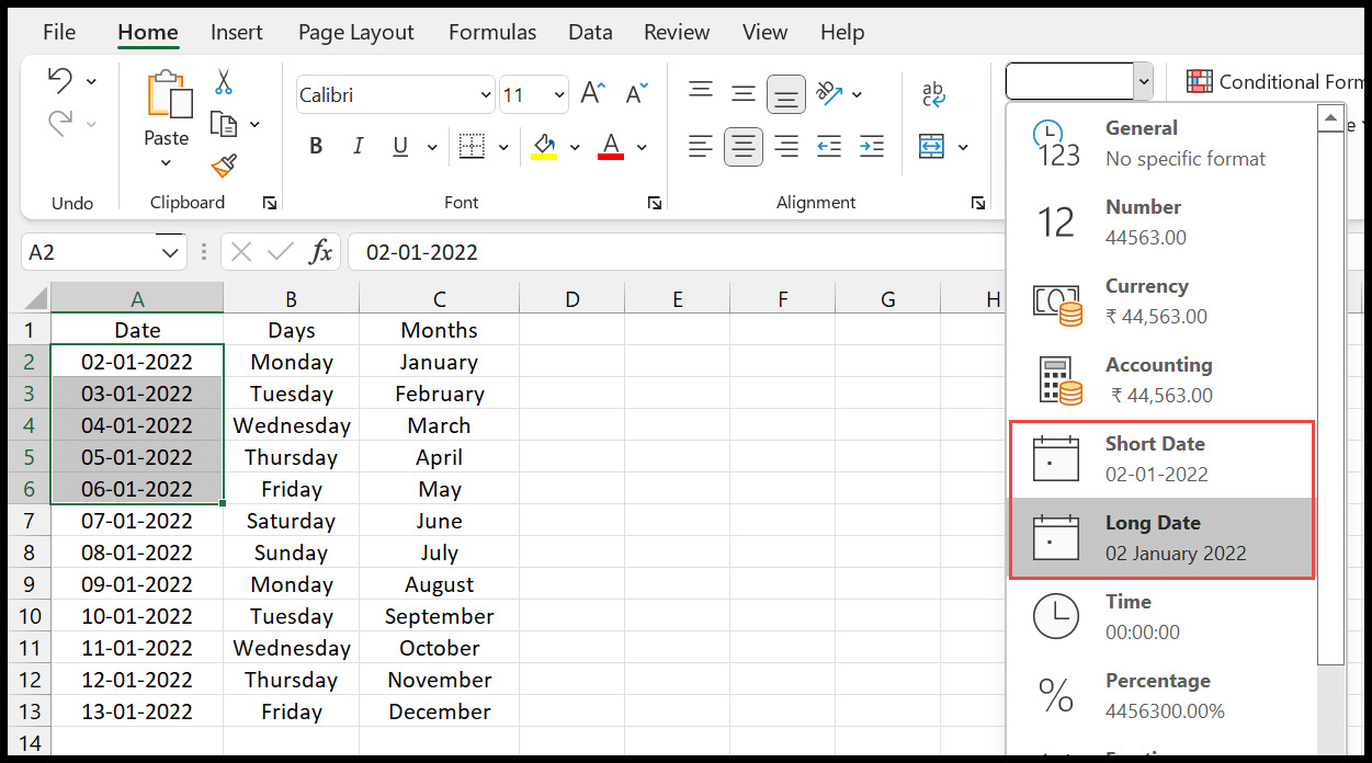
Go to the “Home” tab in the Excel ribbon.
In the “Number” group, you’ll find a dropdown menu with various number formats.
Click on the dropdown arrow to expand the menu.
Navigate to the “Date” section, which will display a list of predefined date formats.
Select the desired date format from the list by clicking on it.

Excel will immediately apply the selected date format to the cells, providing you with a convenient way to switch between different formats. This method is particularly useful when you need to experiment with different date formats quickly or apply common formats like “Short Date” or “Long Date” to your data.

It’s important to note that the available date formats in the Number Format dropdown might vary based on your computer’s regional settings. Excel automatically adjusts the displayed formats to match your regional date preferences, ensuring that you have access to the most relevant options.

By utilizing the Number Format dropdown, you can save time and effort in changing date formats, especially when you need to make quick adjustments to your data presentation.

Now that you understand Method 2, let’s move on to explore another approach for changing date formats in Excel.

Method 3: Using Custom Number Formats

Excel offers a powerful feature known as custom number formats, which allows you to create and apply your own customized date formats. By using this method, you have complete control over how the dates are displayed in your spreadsheet. Here’s how you can use custom number formats to change the date format in Excel:

Select the cells containing the dates that you want to change the format of.
Right-click on the selected cells and click on “Format Cells” from the context menu. Alternatively, you can go to the “Home” tab in the Excel ribbon, click on the “Number” dropdown, and select “More Number Formats” at the bottom of the list.
In the Format Cells dialog box, navigate to the “Number” tab.
On the left side, select “Custom” from the Category list.
In the “Type” field on the right side, enter the custom format code for the desired date format. For example, to display the date in the format of “dd/mm/yyyy,” you would enter “dd/mm/yyyy” in the Type field.
Click “OK” to apply the custom date format to the selected cells.

With custom number formats, you can use a variety of format codes to customize the display of dates. For example:

d: Day of the month without leading zeros (1-31)
dd: Day of the month with leading zeros (01-31)
m: Month as a number without leading zeros (1-12)
mm: Month as a number with leading zeros (01-12)
mmm: Abbreviated month name (Jan-Dec)
mmmm: Full month name (January-December)
yy: Last two digits of the year (00-99)
yyyy: Full year (e.g., 2022)

By combining these format codes, you can create custom date formats that suit your specific needs. Custom number formats offer unparalleled flexibility and allow you to display dates in a format that best represents your data.

Now that you’ve learned about Method 3, let’s move on to explore another method for changing date formats in Excel.

Method 4: Using Text to Columns

If you have dates stored as text in Excel and need to convert them into proper date formats, you can use the Text to Columns feature. This method allows you to split the text into separate columns and convert it into date format simultaneously. Here’s how you can use Text to Columns to change date formats in Excel:

Select the cells containing the text-formatted dates that you want to convert.
Go to the “Data” tab in the Excel ribbon.
In the “Data Tools” group, click on “Text to Columns.”
Select the “Delimited” option if your data is separated by a specific character, such as a comma or a tab. If your data is fixed-width, choose the “Fixed Width” option.
Click “Next” to proceed to the next step.
Select the delimiters or specify the column widths, depending on your data format.
In the “Column data format” section, choose “Date.”
From the “Date” dropdown, select the desired date format that matches the format of your text-formatted dates.
Click “Finish” to complete the Text to Columns process.

The Text to Columns feature will split the text into separate columns based on the specified delimiter or column widths and convert the selected column(s) into proper date formats. This method not only separates the date components but also ensures that Excel recognizes them as valid dates for sorting and calculations.

Using Text to Columns is particularly useful when you need to convert a large amount of text-formatted dates into proper date formats in one go. It saves time and ensures data accuracy, making it an efficient method for changing date formats in Excel.

Now that you’re familiar with Method 4, let’s explore another approach for changing date formats in Excel.

Method 5: Using Formula

Another method for changing date formats in Excel is by using formulas. With formulas, you can manipulate the date values and display them in the desired format. Here’s how you can use formulas to change the date format in Excel:

Create a new column next to the column containing the original dates.
In the first cell of the new column, enter the formula to convert the date format. For example, you can use the TEXT function, which allows you to specify the format you want for the date.
Here’s an example formula: =TEXT(A1, "mm/dd/yyyy"), where A1 is the reference to the cell containing the original date.
Drag the formula down the column to apply it to all the cells where you want to change the date format.

The formula will convert the original date value into text in the specified format. You can customize the format within the formula by using format codes such as “dd” for the day, “mm” for the month, and “yyyy” or “yy” for the year.

Using formulas to change the date format provides flexibility and allows you to precisely control how the dates are displayed. Additionally, formulas can be automated and updated as the original dates change, ensuring that the converted dates stay up to date in real-time.

Now that you understand Method 5, let’s move on to explore one more method for changing date formats in Excel.

Method 6: Using Power Query

Power Query is a powerful tool in Excel that allows you to manipulate and transform data. It provides an efficient way to change date formats by applying transformations to the data before importing it into your worksheet. Here’s how you can use Power Query to change date formats in Excel:

Select the data range that includes the dates you want to change the format of.
Go to the “Data” tab in the Excel ribbon and click on “Get Data” in the “Get & Transform Data” group. Choose the appropriate data source option for your data.
The Power Query Editor will open, displaying a preview of your data.
Select the column containing the dates that you want to change the format of.
Go to the “Transform” tab in the Power Query Editor.
In the “Data Type” section, click on the dropdown arrow of the selected column and choose “Date” or “Date/Time,” depending on your data.
Click on the “More” option within the “Data Type” section to access additional date format options.
Select the desired date format from the list of options, or choose “Custom” to define a custom date format.
Click on the “Close & Load” button in the Power Query Editor to import the transformed data into Excel.

Power Query allows you to convert dates into different formats before importing them into your worksheet. This method is particularly useful when working with large datasets or when you need to perform data transformations on a regular basis.

By using Power Query, you can save time and ensure data integrity by converting the date formats during the import process, without manually modifying the original data.

Now that you’re familiar with Method 6, let’s summarize the different approaches we have explored for changing date formats in Excel.