Text String Definition and Use in Excel

What is a Text String in Excel?

A text string is a sequence of characters or words that are treated as text in Excel. It can include letters, numbers, symbols, and spaces. Text strings are commonly used to represent labels, descriptions, or any data that is purely text-based. Unlike numerical values, Excel treats text strings as alphanumeric data and does not perform calculations or comparisons on them by default.

Text strings in Excel are important for various purposes. They can be used to label columns or rows, provide descriptions in cells, or store any other textual information. Excel treats these text strings as data rather than mathematical entities, allowing users to manipulate, format, and analyze text-based information in a spreadsheet.

Excel recognizes text strings by enclosing them in quotation marks or by explicitly formatting the cells as “Text” format. When a cell contains a text string, Excel displays it exactly as entered, without any automatic formatting or conversion.

It’s important to note that Excel can sometimes interpret numbers or dates as text strings if they are entered in a specific format or if they are preceded by an apostrophe. This allows users to maintain the formatting or prevent automatic conversions when necessary.

Understanding text strings in Excel is crucial for working with data that primarily consists of text-based information. It enables users to perform various operations on text strings, such as extracting specific characters, combining multiple strings, changing case, and more. By utilizing the power of text functions and formulas, Excel users can efficiently manipulate and analyze textual data to derive meaningful insights.

How to Enter a Text String in Excel

Entering a text string in Excel is a simple process. Here are a few methods you can use:

Directly typing: The most straightforward way to enter a text string is by directly typing it into a cell. Start by selecting the desired cell, then type the text string. Excel will display the text as you enter it, surrounding it with quotation marks if necessary.
Preceding with an apostrophe: Another way to enter a text string is by preceding it with an apostrophe (‘). For example, if you want to enter “Hello World” as a text string, type it as ‘Hello World. The apostrophe tells Excel to treat the content as text, even if it resembles a number or date format.
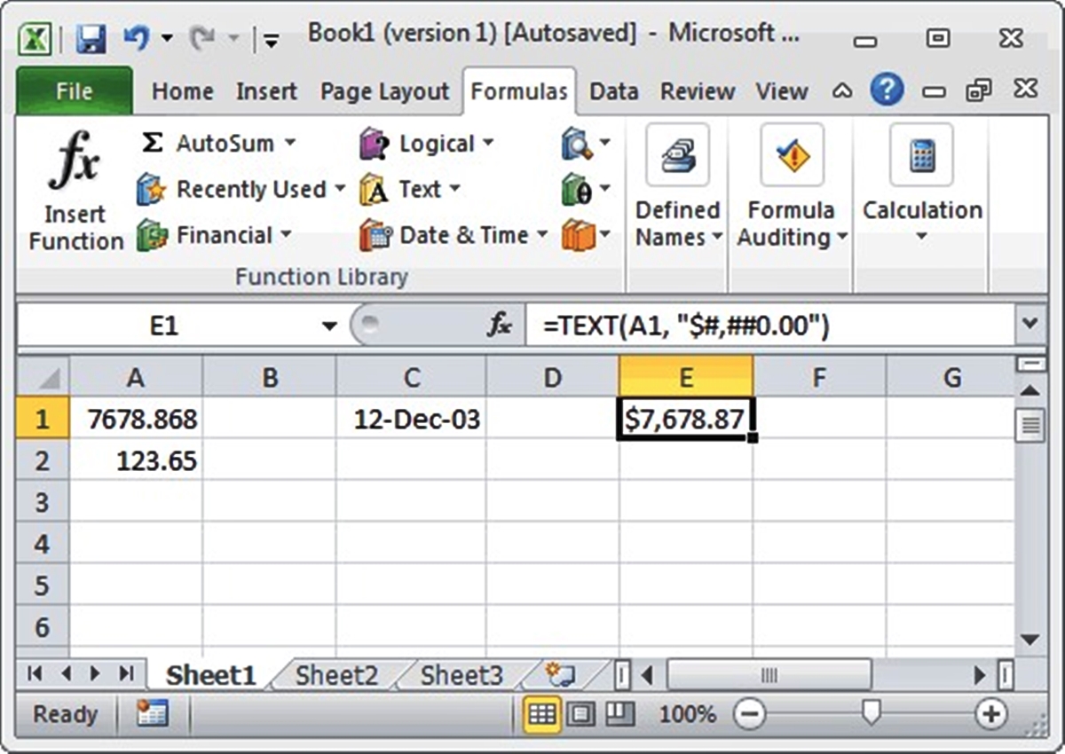
Using text formulas: Excel provides several text formulas that can be used to enter text strings dynamically. For example, the CONCATENATE function allows you to combine multiple text strings into a single cell. The TEXT function allows you to format numerical values as text strings with specific formatting rules.

It’s important to note that if a text string contains quotation marks, you need to use double quotation marks (“”) to represent a single quotation mark within the text. For example, to enter the text string “He said, “Hello!”” you would type it as “He said, “”Hello!””.”

Additionally, Excel has a feature called AutoCorrect that can automatically correct common typing mistakes and convert certain text strings into other data types. To prevent AutoCorrect from altering your text strings, you can either disable it or format the cells as “Text” before entering the text strings.

By using these methods, you can effortlessly enter text strings in Excel and ensure that they are recognized and treated as text rather than other data types.

Manipulating Text Strings with Formulas

Excel provides a variety of powerful formulas to manipulate and transform text strings. These formulas can be used to extract specific characters, combine text strings, remove unwanted characters, change the case of text, find and replace text, and more.

Here are some commonly used text functions in Excel:

LEFT: This function allows you to extract a specified number of characters from the beginning of a text string. For example, to extract the first 3 characters from the text string “Excel”, you would use the formula =LEFT(“Excel”, 3), which returns “Exc”.
RIGHT: Similar to the LEFT function, the RIGHT function extracts a specified number of characters from the end of a text string. For instance, =RIGHT(“Excel”, 2) would return “el”.
MID: The MID function extracts a specific number of characters from a text string, starting from a specified position. For example, =MID(“Excel”, 2, 3) would extract the characters “xce” from the string.
CONCATENATE: This function combines multiple text strings into one. For instance, =CONCATENATE(“Hello”,” “,”World”) would result in “Hello World”. Alternatively, you can use the ampersand (&) operator to achieve the same result, like “Hello” & ” ” & “World”.
LOWER and UPPER: These functions change the case of text. LOWER converts text to lowercase, while UPPER converts it to uppercase. For example, =LOWER(“Hello”) would return “hello”.
SUBSTITUTE: The SUBSTITUTE function replaces specific text in a string with new text. For example, =SUBSTITUTE(“Apples and Oranges”, “Apples”, “Bananas”) would replace the word “Apples” with “Bananas”, resulting in “Bananas and Oranges”.
FIND and REPLACE: These functions help locate and replace specific text within a larger text string. FIND returns the position of the text, while REPLACE replaces it with new text. For example, =FIND(“World”, “Hello World”) returns 7, and =REPLACE(“Hello World”, 7, 5, “Universe”) replaces “World” with “Universe”.

By utilizing these text formulas, you can perform a wide range of operations on text strings in Excel. Whether it’s extracting specific characters, combining text, changing case, or manipulating text using your own custom logic, these formulas provide the flexibility and power to tailor your text strings to your specific needs.

Extracting Characters from a Text String

In Excel, you can extract specific characters from a text string using various methods and functions. This can be useful when you need to retrieve certain portions of a larger text string, such as extracting the first name from a full name, or retrieving the area code from a phone number.

Here are a few methods for extracting characters from a text string:

LEFT Function: The LEFT function allows you to extract a specified number of characters from the leftmost side of a text string. For example, to extract the first 3 characters from the text string “Excel”, you would use the formula =LEFT(“Excel”, 3), which would return “Exc”.
RIGHT Function: Conversely, the RIGHT function extracts a specified number of characters from the rightmost side of a text string. For instance, =RIGHT(“Excel”, 2) would extract the last 2 characters, resulting in “el”.
MID Function: The MID function can be used to extract a specific number of characters from within a text string. It requires the starting position and the number of characters to extract. For example, =MID(“Hello World”, 7, 5) would extract “World” from the string.
FIND and SEARCH Functions: The FIND and SEARCH functions are useful when you need to extract characters based on a specific text pattern or delimiter. FIND returns the starting position of a text within another text, while SEARCH is case-insensitive. Using these functions in combination with the MID function allows you to extract characters based on a pattern. For example, =MID(“John-Doe”, FIND(“-“, “John-Doe”) + 1, LEN(“John-Doe”)) would extract “Doe” from the string.
Text to Columns Feature: The Text to Columns feature in Excel allows you to split a text string into different columns based on a delimiter. This can be useful when you have structured data, such as addresses or CSV files, and want to separate the different components into separate columns.

By utilizing these methods and functions, you can easily extract specific characters or substrings from text strings in Excel. Whether you need to retrieve a specific portion of a string or split a string into different parts, Excel provides a range of tools to help you accomplish these tasks efficiently.

Concatenating Text Strings

Concatenation is the process of combining multiple text strings into one. In Excel, you can concatenate text strings using different methods and functions, allowing you to create customized text outputs.

Here are a few methods for concatenating text strings in Excel:

Concatenation Operator: The simplest way to concatenate text strings is by using the ampersand (&) operator. For example, to combine the texts “Hello” and “World”, you would write “Hello” & “World”, resulting in the concatenated string “HelloWorld”. You can also include space or other characters by adding them within quotes, like “Hello” & ” ” & “World” to yield “Hello World”.
CONCATENATE Function: Excel also provides a CONCATENATE function that concatenates multiple text strings. For instance, =CONCATENATE(“Hello”, ” “, “World”) would yield the same result as “Hello” & ” ” & “World”. This function allows you to join more than two text strings together easily, simply by including additional arguments.
TEXTJOIN Function: The TEXTJOIN function is particularly useful when you want to concatenate a range of cells or include a delimiter between the concatenated text strings. For example, =TEXTJOIN(“, “, TRUE, A1:A3) would concatenate the values in cells A1, A2, and A3, separated by a comma and a space.
Using Formulas and Text Functions: Excel’s formulas and text functions can be combined to concatenate text strings dynamically. For instance, you can use the CONCATENATE function with other functions, like =CONCATENATE(“Hello”, “, “, UPPER(“world”)), which would result in “Hello, WORLD”. This allows you to incorporate calculations and manipulate text strings while joining them together.
Joining Text with Line Breaks: If you want to concatenate text strings with line breaks, you can use the CHAR function combined with concatenation. For example, =A1 & CHAR(10) & A2 would join the values in cells A1 and A2, with a line break between them.

By using these methods and functions, you can concatenate text strings in Excel to create customized outputs tailored to your specific needs. Whether you need to combine simple text strings, include delimiters, or join text strings from a range of cells, Excel provides various tools to help you perform these operations efficiently.

Removing Unwanted Characters from a Text String

When working with text strings in Excel, you may encounter situations where you need to remove unwanted characters or specific parts of a string. Fortunately, Excel provides several methods and functions to accomplish this task effectively.

Here are a few methods for removing unwanted characters from a text string in Excel:

REPLACE Function: The REPLACE function allows you to replace specific characters or substrings within a text string. By specifying the starting position and the number of characters to replace, you can remove unwanted characters. For example, you can use =REPLACE(“Hello World”, 6, 6, “”) to remove the word “World” and leave only “Hello” in the cell.
SUBSTITUTE Function: The SUBSTITUTE function replaces specific instances of a character or substring within a text string. By using an empty string (“”) as the replacement text, you can effectively remove unwanted characters. For example, =SUBSTITUTE(“Hello World”, ” “, “”) would remove all spaces from the text string.
LEFT, RIGHT, and MID Functions: The LEFT, RIGHT, and MID functions can be used to extract specific portions of a text string, effectively removing unwanted characters. By specifying the desired number of characters or the starting position, you can extract the clean part of the text string. This is particularly useful when dealing with fixed-length formats or when unwanted characters occur in predictable positions.
TRIM Function: The TRIM function is especially useful when dealing with leading or trailing spaces in a text string. It removes extra spaces between words and removes leading and trailing spaces. For example, =TRIM(” Hello “) would remove the extra spaces and return “Hello”.
Using Formulas and Text Functions: Excel’s formulas and text functions can be combined to remove unwanted characters from a text string. For example, you can use functions like SUBSTITUTE, REPLACE, LEFT, RIGHT, and MID, in combination with logical functions like IF or FIND, to implement custom logic and remove specific characters or substrings based on specific conditions or patterns.

By utilizing these methods and functions, you can effectively remove unwanted characters or parts of a text string in Excel. Whether you need to replace specific characters, remove spaces, or extract clean portions of a text string, Excel provides a range of tools to help you perform these operations efficiently.

Changing the Case of Text in Excel

In Excel, you can easily change the case of text strings, converting them to uppercase, lowercase, or title case. This can be helpful when you need to standardize the formatting of text or perform specific analyses based on the case of the text.

Here are a few methods to change the case of text in Excel:

UPPER Function: The UPPER function converts text to uppercase. For example, =UPPER(“hello”) would result in “HELLO”. You can apply this function to individual cells or to a range of cells using a formula or a copy-paste operation.
LOWER Function: The LOWER function converts text to lowercase. For instance, =LOWER(“HELLO”) would yield “hello”. Similar to the UPPER function, you can apply the LOWER function to single cells or a range of cells.
PROPER Function: The PROPER function converts text to title case, capitalizing the first letter of each word. For example, =PROPER(“hello world”) would result in “Hello World”.
Using Formulas and Text Functions: Excel’s formulas and text functions can be combined to manipulate the case of the text strings based on custom logic. For example, you can use functions like UPPER, LOWER, FIND, MID, and SUBSTITUTE in conjunction with logical functions like IF to perform case transformations based on specific criteria. This allows you to implement more advanced case-changing operations.
Using the Ribbon Option: Excel also provides a convenient option to change the case of text through the ribbon interface. Select the cells containing the text, go to the “Home” tab, and choose the desired case transformation from the “Font” section in the ribbon (e.g., “Aa” for uppercase, “aa” for lowercase, or “AaBbCc” for title case).

By using these methods and functions, you can easily change the case of text strings in Excel. Whether you need to convert text to uppercase for consistency, lowercase for aesthetic purposes, or title case for proper capitalization, Excel provides the necessary tools to achieve these transformations efficiently.

Finding and Replacing Text in Excel

Excel provides powerful features to find and replace specific text within a worksheet or a range of cells. Whether you need to update data, correct mistakes, or make bulk changes, these tools can save you time and effort.

Here are a few methods for finding and replacing text in Excel:

Find and Replace: The Find and Replace tool in Excel allows you to locate specific text within a worksheet or a selected range and replace it with new text. You can access this feature by pressing Ctrl + F or navigating to the “Home” tab and clicking on the “Find & Select” button. This opens a dialog box where you can enter the text to find and the text to replace it with.
Using the Find and Replace dialog box: The Find and Replace dialog box provides additional options, such as case-sensitivity, finding whole words only, and searching within formulas. This allows for more precise and controlled replacements. To access the dialog box, use the shortcut Ctrl + H or navigate to the “Home” tab and click on the “Find & Select” button, then choose “Replace” from the drop-down menu.
Replace Within Specific Cells or Formulas: You can also use the “Replace” function to specify the range of cells or formulas to search within. For example, you can replace text only within a specific column by selecting that column before using the Find and Replace tool. Similarly, when using the REPLACE function, you can specify a cell reference or a formula to replace text within a particular cell.
Replacing Multiple Instances: If you have multiple instances of the same text within a cell and want to replace all of them, you can use the SUBSTITUTE function. This function replaces all occurrences of a specific string with another string. For instance, =SUBSTITUTE(“Hello, hello, hello!”, “hello”, “hi”) would replace all instances of “hello” with “hi”, resulting in “Hello, hi, hi!”
Using Wildcards: Excel’s Find and Replace tool supports the use of wildcards, which are special characters that represent sets of characters. This allows for more flexible and advanced searches. For example, you can use an asterisk (*) as a wildcard to find and replace multiple characters. For instance, searching for “app*” would find “apple”, “application”, and “applesauce”.

By utilizing these methods and tools, you can efficiently find and replace specific text in Excel. Whether you need to correct errors, update data, or make bulk changes, Excel provides a range of options to help you perform these tasks accurately and speedily.

Using Text to Columns Feature

Excel’s “Text to Columns” feature allows you to split a single column of text into multiple columns based on a delimiter or a fixed width. This can be useful when you have data that is combined in a single cell or when you import data from external sources that need to be separated into individual columns.

Here’s how you can use the “Text to Columns” feature in Excel:

Delimited Text: If your data is delimited, meaning that there is a specific character or symbol separating the information, you can use this option. For example, if you have a column containing “First Name, Last Name” with a comma separating the two names, you can choose the “Delimited” option and specify the delimiter as a comma. Excel will split the text into two columns, one for the first name and one for the last name.
Fixed Width Text: If your data has a consistent pattern where the information is of fixed width, such as a specific number of characters for each column, you can choose the “Fixed Width” option. You’ll need to manually set the breakpoints by clicking and dragging the vertical lines to match the width of the data. Excel will split the text into separate columns based on the defined widths.
Additional Options: Within the “Text to Columns” dialog box, you can choose additional options based on your specific needs. These options include selecting the data format for each column, skipping columns, and specifying advanced settings like decimal and thousands separators.
Preview and Adjust: Before finalizing the splitting process, Excel provides a preview of how the data will be separated into columns. You can review and adjust the column widths, delimiters, and other settings to ensure that the data is split correctly.
Applying the Changes: Once you are satisfied with the preview, click “Finish” to apply the changes. Excel will separate the text into individual columns according to your chosen method. The original column will be replaced by the newly created columns.

The “Text to Columns” feature in Excel is a powerful tool for splitting text into separate columns based on a delimiter or a fixed width. It allows you to efficiently organize and structure your data, making it easier to analyze and work with in Excel.

Importing and Exporting Text Files in Excel

Excel provides functionality to import and export text files, allowing you to seamlessly work with external data in your spreadsheets.

Here’s how you can import and export text files in Excel:

Importing Text Files: To import a text file into Excel, go to the “Data” tab and click on “From Text” or “Get External Data”. Select the desired text file from your computer and follow the import wizard. The import wizard allows you to specify the data delimiter, the text encoding, and the column format. Once completed, Excel will import the text file into a new or existing worksheet, placing the data in separate columns.
Exporting Text Files: To export data from Excel to a text file, select the range of cells you want to export. Go to the “File” tab, choose “Save As”, and select the desired location for the exported text file. In the “Save As” dialog box, choose the text file format (such as CSV or TXT). Excel will convert the selected range of cells into text format and save it as a text file that can be opened in other applications.
Working with Delimited Text: When importing or exporting text files, Excel recognizes delimiter-separated values, such as comma-separated values (CSV) or tab-delimited files. Delimiters can be specified during the import or export process, allowing Excel to properly separate data into columns.
Formatting and Text Import Wizard: During the import process, Excel provides the Text Import Wizard to handle different types of delimiters, text qualifiers, and column data formats. The wizard allows you to specify the data layout and preview the results before importing the text file.
Refreshing Imported Data: If you have imported a text file into Excel and later make changes to the text file, you can use the “Refresh” or “Refresh All” options to update the imported data in Excel. This ensures that your Excel worksheet reflects the most current version of the text file.

Importing and exporting text files in Excel offers a convenient way to integrate external data into your spreadsheets and collaborate with other applications. Whether you need to analyze data from different sources or share data with others, Excel’s import and export functionality simplifies the process and enhances data interoperability.