How To Use OpenOffice Calc Formulas

Basics of Formulas

Formulas are the heart and soul of spreadsheet applications like OpenOffice Calc. They allow you to perform calculations, manipulate data, and automate tasks. Understanding the basics of formulas is crucial for harnessing the full power of this tool.

At its core, a formula is an expression that starts with an equal sign (=) and consists of one or more functions, operators, and cell references. Cell references are used to refer to specific cells within a spreadsheet and are denoted by the column letter and row number, such as A1 or B4.

Operators are symbols that perform mathematical or logical operations. Common operators include addition (+), subtraction (-), multiplication (*), division (/), and exponentiation (^). You can use these operators in formulas to perform calculations on values or cell references.

For example, if you want to calculate the sum of the values in cells A1 and A2, you can use the formula =A1+A2. This formula adds the values in the cells A1 and A2 and displays the result in the cell where the formula is entered.

In addition to using operators, you can also incorporate functions into your formulas. Functions are predefined formulas that perform specific tasks. They can range from simple calculations like finding the average or sum of a range of cells to more complex tasks like determining the maximum or minimum value.

To use a function, you need to specify its name followed by a set of parentheses (). Within the parentheses, you can include arguments, which are the values or cell references that the function operates on.

For example, the function SUM(A1:A5) calculates the sum of the values in the range A1 to A5. The result is displayed in the cell where the formula is entered.

It’s important to note that formulas are dynamic and can update automatically when the referenced cells change. This makes it easy to perform calculations on large sets of data and keep your spreadsheets up to date.

By understanding the basics of formulas in OpenOffice Calc, you can unlock the potential to automate calculations, manipulate data, and streamline your workflows. Experiment with different functions, operators, and cell references to explore the possibilities and make the most of this powerful tool.

Understanding Cell References

In OpenOffice Calc, cell references are used to refer to specific cells within a spreadsheet. They allow you to manipulate and perform calculations on the data contained in those cells. Understanding how cell references work is essential for creating accurate and dynamic formulas.

There are three types of cell references: relative, absolute, and mixed references.

A relative reference is the default type of reference in Calc. When you copy a formula with relative references to another cell, the references adjust automatically based on the new location of the formula. For example, if you have a formula that adds the values of cells A1 and A2 (like =A1+A2), and you copy it to cell B1, the formula will adjust to =B1+B2. This relative adjustment allows you to easily apply a formula to multiple cells.

An absolute reference is used when you want a specific cell reference to remain constant, regardless of where the formula is copied or moved. To create an absolute reference, you use the dollar sign ($) before the column letter, the row number, or both. For example, if you have a formula that calculates the percentage of a total, like =A1/$B$1, the absolute reference $B$1 ensures that the denominator remains fixed at cell B1, even if the formula is copied to other cells.

A mixed reference is a combination of relative and absolute references. You can fix either the row or column while allowing the other to adjust. For example, if you have a formula that multiplies the values in column A by a fixed value in cell $B$1, you can use the mixed reference $B1 or B$1. The column letter will adjust when copied, but the row number or column letter will remain constant, respectively.

To switch between different types of references, you can use the F4 key on your keyboard while editing a formula. Pressing F4 toggles between relative, absolute, and mixed references.

Understanding cell references is crucial for creating complex formulas and performing calculations across multiple cells or ranges. By mastering the various reference types and knowing when to use them, you can build powerful and flexible formulas to analyze and manipulate your data effectively.

Using Basic Operators

Operators are symbols or characters used in formulas to perform mathematical or logical operations in OpenOffice Calc. They allow you to manipulate data and perform calculations within your spreadsheets. Understanding and using basic operators is essential for creating formulas that yield the desired results.

There are several basic operators that you can use in Calc:

Addition (+): The addition operator adds two or more values together. For example, the formula =A1+B1 adds the values in cells A1 and B1.
Subtraction (-): The subtraction operator subtracts one value from another. For example, the formula =A1-B1 subtracts the value in cell B1 from cell A1.
Multiplication (*): The multiplication operator multiplies two or more values. For example, the formula =A1*B1 multiplies the values in cells A1 and B1.
Division (/): The division operator divides one value by another. For example, the formula =A1/B1 divides the value in cell A1 by cell B1.
Exponentiation (^): The exponentiation operator raises a number to a power. For example, the formula =A1^B1 raises the value in cell A1 to the power of cell B1.

These basic operators can be combined within formulas to perform more complex calculations. For example, the formula =A1+B1*C1 calculates the sum of the value in cell A1 and the product of cells B1 and C1.

It’s important to note that operators follow a specific order of precedence. This means that certain operators are evaluated before others. If you want to change the order of evaluation, you can use parentheses () to group operations. Anything within parentheses is evaluated first. For example, the formula =(A1+B1)*C1 adds the values in cells A1 and B1, and then multiplies the result by the value in cell C1.

Understanding and utilizing basic operators in your formulas allows you to perform calculations, manipulate data, and customize the behavior of your spreadsheets in OpenOffice Calc effectively. Experiment with different combinations of operators to achieve the desired results in your calculations.

Performing Mathematical Operations

OpenOffice Calc offers a range of mathematical operations that you can perform within your spreadsheets. These operations allow you to manipulate numerical data and perform calculations to analyze and interpret your data effectively.

Calc supports the basic mathematical operations such as addition (+), subtraction (-), multiplication (*), and division (/). These operations can be used with numeric values or cell references to perform calculations. For example, you can use the formula =A1 + B1 to add the values in cells A1 and B1.

In addition to the basic operations, Calc also supports more advanced mathematical functions. These functions can be used to perform operations such as finding the square root, calculating logarithms, trigonometric functions, and rounding numbers.

For example, to calculate the square root of a number, you can use the SQRT function. The formula =SQRT(A1) will return the square root of the value in cell A1.

Calc also provides functions for rounding numbers. The ROUND function allows you to round a number to a specified number of decimal places. For example, the formula =ROUND(A1, 2) will round the value in cell A1 to 2 decimal places.

Another useful mathematical function in Calc is the SUM function. This function allows you to calculate the sum of a range of cells. For example, the formula =SUM(A1:A5) will add the values in cells A1 to A5 and return the total sum.

Calc also supports the use of mathematical constants such as pi and e. These constants can be used in formulas to perform calculations. For example, the formula =2 * PI() will multiply the value of pi by 2.

By utilizing the mathematical operations and functions available in OpenOffice Calc, you can perform a wide range of calculations and manipulate numerical data within your spreadsheets. Experiment with different functions and operations to analyze your data effectively and gain valuable insights.

Using Functions

Functions are predefined formulas that perform specific tasks in OpenOffice Calc. They allow you to automate calculations, manipulate data, and perform complex operations without needing to write the entire formula manually. Understanding how to use functions is essential for efficient and accurate spreadsheet calculations.

In Calc, functions are built-in and categorized based on their respective purposes. You can find functions for mathematical operations, statistical analysis, text manipulation, date and time calculations, and more.

For example, the SUM function is commonly used to calculate the sum of a range of cells. To use the SUM function, you would enter =SUM(A1:A5), where A1:A5 represents the range of cells you want to add. The result of the sum would be displayed in the cell where the formula is entered.

Functions can have multiple arguments. For instance, the IF function is used for conditional calculations. It takes three arguments: a logical expression, a value if the expression is true, and a value if the expression is false. The formula =IF(A1>10, “Yes”, “No”) would display “Yes” if the value in cell A1 is greater than 10, and “No” if it is not.

Calc also supports nested functions, which means you can use one function as an argument within another function. This allows you to combine multiple functions to achieve more complex calculations. For example, the formula =ROUND(SUM(A1:A5)/COUNT(A1:A5), 2) uses the ROUND function and the SUM function together to calculate the average of the values in the range A1 to A5 and rounds the result to two decimal places.

It’s important to understand the syntax and parameters of each function you use. Refer to the Calc documentation or online resources to explore the available functions and their specific purposes.

By leveraging the power of built-in functions in OpenOffice Calc, you can streamline your calculations, automate tasks, and handle complex operations efficiently. Experiment with different functions to discover the wide range of possibilities and enhance your spreadsheet capabilities.

Syntax of Functions

The syntax of a function refers to the specific structure and arrangement of its components within a formula. Understanding the syntax is crucial for correctly using and incorporating functions in your calculations in OpenOffice Calc. Although the syntax may vary slightly depending on the function, there are some common elements to be aware of.

The basic syntax of a function consists of the function name followed by a set of parentheses (). Within the parentheses, you provide the necessary arguments, separated by commas if there are multiple arguments. Arguments can be values, cell references, or even other functions.

For example, the syntax for the SUM function looks like this: =SUM(argument1, argument2, …). You would replace “argument1, argument2, …” with the relevant values or cell references that you want to include in the sum.

Some functions also require additional parameters or options. These parameters modify how the function operates or specify certain conditions. Depending on the function, these parameters can be included within the parentheses along with the arguments or specified separately.

For instance, the syntax for the IF function includes three parameters: =IF(logical_expression, value_if_true, value_if_false). The logical_expression is the condition that the function evaluates, while value_if_true and value_if_false represent the results to display based on the evaluation of the logical_expression.

It’s important to use the correct syntax and provide the required arguments in the right order. Incorrect syntax can result in errors or unexpected outcomes in your formulas. Be mindful of any specific requirements or limitations mentioned in the documentation for each function.

Furthermore, Calc supports multiple languages and the syntax for functions can vary depending on the language set in your application. If you are using localized versions, ensure you use the appropriate syntax for your language.

When using functions, it can be helpful to utilize the built-in function wizard or autocomplete feature in Calc. These tools guide you through the process of entering functions correctly by providing a list of available functions, descriptions, and parameters.

By understanding the syntax of functions in OpenOffice Calc, you can effectively incorporate them into your formulas. Pay attention to the function name, parentheses, arguments, and any additional parameters required. With proper syntax, you can unleash the full potential of functions to perform various calculations and manipulate data within your spreadsheets.

Commonly Used Functions

In OpenOffice Calc, there are numerous functions available to perform various calculations, manipulate data, and automate tasks within your spreadsheets. Understanding and utilizing commonly used functions can greatly enhance your productivity and enable you to perform complex operations efficiently. Here are some of the most commonly used functions in Calc:

SUM: This function calculates the sum of a range of cells. For example, SUM(A1:A5) adds up the values in cells A1 to A5.
AVERAGE: The AVERAGE function calculates the average value of a range of cells. For instance, AVERAGE(B1:B10) returns the average of the values in cells B1 to B10.
MAX and MIN: These functions return the maximum and minimum values, respectively, within a range of cells. MAX(A1:A5) gives you the highest value in cells A1 to A5, while MIN(B1:B10) gives you the lowest value in cells B1 to B10.
COUNT: The COUNT function counts the number of cells that contain numeric values within a range. COUNT(C1:C10) gives you the count of cells with numeric values in cells C1 to C10.
IF: The IF function allows you to perform conditional calculations. It evaluates a logical expression and returns different values based on the result. For example, IF(A1>10, “Yes”, “No”) displays “Yes” if the value in cell A1 is greater than 10, and “No” if it is not.
CONCATENATE: The CONCATENATE function combines multiple strings of text. CONCATENATE(A1, ” “, B1) concatenates the values in cells A1 and B1, with a space in between.
DATE and TODAY: The DATE function allows you to create a date based on specified year, month, and day values. TODAY returns the current date. These functions are useful for date calculations and tracking purposes.
TEXT: The TEXT function allows you to format numeric values as text. It is useful for displaying numbers with specific formats or converting them to a specific text format.

These are just a few examples of commonly used functions in Calc. Remember that Calc offers a wide range of other functions that can handle various tasks such as text manipulation, statistical analysis, financial calculations, and more. Familiarize yourself with these functions to utilize the full potential of Calc and streamline your spreadsheet operations.

Nesting Functions

In OpenOffice Calc, you can nest functions by using one function as an argument within another function. This technique allows you to perform complex calculations and combine multiple functions to achieve the desired results. Nesting functions offers a powerful way to manipulate data and automate tasks within your spreadsheets.

To nest functions, you simply include the inner function as an argument within the parentheses of the outer function. The result of the inner function serves as the input for the outer function.

For example, let’s say you want to calculate the average of a range of cells, but you only want to include values that are greater than a certain threshold. You can achieve this by nesting the AVERAGE function within the IF function. The formula would look like this: =AVERAGE(IF(A1:A10 > 5, A1:A10, “”))

In this formula, the IF function checks if each value in the range A1 to A10 is greater than 5. If it is, it includes the value in the calculation; otherwise, it treats it as an empty string. The result is then passed to the AVERAGE function, which calculates the average of the qualifying values.

You can nest functions to multiple levels if needed. This means that the inner function can itself contain another nested function. However, it’s important to make sure that the parentheses are correctly balanced and the functions are nested in the desired order.

Nesting functions allows you to create more sophisticated calculations and perform advanced data manipulation. You can combine functions for mathematical operations, logical tests, text manipulations, and more to achieve specific results.

While nesting functions can be powerful, it’s important to maintain clarity and ensure the formula remains understandable. Excessive nesting can make formulas complex and difficult to troubleshoot. Consider breaking down complex formulas into smaller parts or utilizing helper columns for better readability and maintainability.

Experiment with nesting functions in OpenOffice Calc to harness the full potential of their capabilities. By combining functions, you can perform intricate calculations and automate tasks, making your spreadsheet operations more efficient and dynamic.

Working with Ranges

In OpenOffice Calc, ranges are groups of cells that are used together in formulas and calculations. Working with ranges allows you to perform operations on a set of cells, manipulate data collectively, and create dynamic formulas that adapt to changes in your spreadsheet.

Ranges can be specified using a combination of column letters and row numbers. For example, A1:B5 represents a rectangular range that includes cells from A1 to B5.

You can use ranges in a variety of ways:

Performing calculations: Ranges are commonly used with functions to perform calculations on multiple cells at once. For example, =SUM(A1:A5) adds up the values in the range A1 to A5.
Applying formatting: Ranges are useful for applying formatting options to multiple cells simultaneously. You can select a range of cells and modify properties like font, color, alignment, and more.
Copying and pasting: Using ranges allows you to copy and paste data more efficiently. You can select a range, copy it, and then paste it into multiple cells, replicating the data quickly.
Performing operations on subsets: Ranges provide a way to extract and analyze specific subsets of your data. By referencing a range in formulas or functions, you can perform operations and calculations on only the desired cells.

Calc provides additional tools for working with ranges:

Range Names: You can assign names to ranges to make your formulas more understandable and easier to manage. Range names can be used in place of cell references in formulas for better clarity.
Range Calculations: Using the Define Names feature, you can define ranges that automatically adjust their size based on the data entered. This allows formulas to adapt to changes in the range without requiring manual adjustments.
Conditional Formatting: Ranges can be used to apply conditional formatting to highlight specific cells based on certain criteria. This is useful for visually identifying patterns or outliers within your data.

Understanding how to work with ranges in OpenOffice Calc is essential for effective spreadsheet management and data analysis. By utilizing ranges in your formulas, calculations, formatting, and data manipulation tasks, you can streamline your workflow and make your spreadsheets more dynamic and efficient.

Using Conditional Statements

In OpenOffice Calc, conditional statements allow you to perform calculations and make decisions based on specific conditions. Conditional statements are powerful tools that enable you to automate processes, analyze data, and manipulate information in your spreadsheets.

The most commonly used conditional statement in Calc is the IF function. The IF function evaluates a logical expression and returns different values based on whether the condition is true or false. The basic syntax of the IF function is: =IF(logical_expression, value_if_true, value_if_false).

The logical_expression is a condition that you want to evaluate. It can be a simple comparison (e.g., A1 > 10) or a more complex combination of logical operators and functions. If the logical_expression is true, the value_if_true is returned; otherwise, the value_if_false is returned.

For example, let’s say you have a column of sales data in cells A1 to A5, and you want to display “Yes” if a value is greater than 1000 and “No” if it is not. You can use the IF function like this: =IF(A1 > 1000, “Yes”, “No”). This formula will check if the value in cell A1 is greater than 1000. If it is, the word “Yes” will be displayed; otherwise, “No” will be displayed.

Conditional statements can also be combined with other functions and nested within each other to create complex calculations. For example, you can use multiple IF functions to define multiple conditions and outcomes within a single formula.

Here’s an example: =IF(A1 > 1000, “High”, IF(A1 > 500, “Medium”, “Low”)). In this formula, if the value in cell A1 is greater than 1000, it will display “High”; if it is greater than 500, it will display “Medium”; otherwise, it will display “Low”. This allows you to categorize your data based on different conditions.

Conditional statements can also be combined with other functions to perform more sophisticated calculations. You can use logical operators such as AND, OR, and NOT to create complex logical expressions within your formulas.

By using conditional statements effectively in OpenOffice Calc, you can automate decision-making processes, analyze and summarize data based on specific conditions, and create dynamic and customized spreadsheets.

Using Logical Functions

Logical functions are valuable tools in OpenOffice Calc that allow you to perform calculations and make decisions based on logical conditions. They enable you to evaluate data, test multiple conditions, and automate processes within your spreadsheets.

Calc offers several commonly used logical functions:

AND: The AND function evaluates multiple conditions and returns TRUE if all conditions are true; otherwise, it returns FALSE. For example, the formula =AND(A1>10, B1<20) would return TRUE if the values in cells A1 and B1 satisfy both conditions. Otherwise, it would return FALSE.
OR: Similarly, the OR function evaluates multiple conditions and returns TRUE if at least one condition is true; otherwise, it returns FALSE. For example, =OR(A1>10, B1>20) returns TRUE if either of the two conditions is true.
NOT: The NOT function reverses the logical value of a condition. It returns TRUE if the condition is false, and vice versa. For example, =NOT(A1>10) returns TRUE if the value in cell A1 is not greater than 10.
IF: The IF function, as mentioned earlier, is a powerful logical function that allows you to make decisions based on conditions. It evaluates a logical expression and returns different values depending on whether the condition is true or false.

Logical functions can be nested to create more complex calculations and decision-making processes. By combining logical functions, you can evaluate multiple conditions and create intricate logic in your formulas.

Logical functions are particularly useful when combined with conditional statements (such as the IF function) for more advanced data analysis and decision-making. By using logical functions, you can automate data classification, filter data based on specific criteria, and perform calculations on subsets of data.

When using logical functions, it’s important to ensure that your conditions are properly constructed and that they evaluate as expected. Pay attention to the logical operators used (such as >, <, =) and make sure they align with your intended comparisons and outcomes.

Overall, logical functions enhance the flexibility and power of your spreadsheet calculations. They enable you to evaluate data programmatically, automate decision-making processes, and create dynamic formulas that adapt to changes in your data.

Using Date and Time Functions

Date and time functions in OpenOffice Calc allow you to perform calculations, manipulate, and format date and time values within your spreadsheets. These functions are particularly useful for tracking deadlines, calculating durations, and analyzing time-based data. Let’s explore some commonly used date and time functions:

TODAY: The TODAY function returns the current date, updating automatically each day. This function is helpful for tasks that require tracking the current date without manual intervention.
NOW: The NOW function returns both the current date and time. It updates automatically each time the spreadsheet is calculated or recalculated.
DATE: The DATE function constructs a date by specifying the year, month, and day as separate arguments. For example, the formula =DATE(2022, 12, 31) would return the date December 31, 2022.
TIME: The TIME function constructs a time value by specifying the hour, minute, and second as separate arguments. For instance, =TIME(9, 30, 0) would represent 9:30 AM.
DATEDIF: The DATEDIF function calculates the difference between two dates in years, months, or days. It’s useful for determining the duration between two specific dates.
MONTH: The MONTH function extracts the month component from a date or serial number. For example, =MONTH(A1) would return the month value of the date in cell A1.
YEAR: The YEAR function extracts the year component from a date or serial number. For instance, =YEAR(A1) would retrieve the year value from cell A1.
NOW(), TODAY() Format Functions: These functions format the date and time values using various predefined formats such as “Short Date,” “Long Date,” “Short Time,” and “Long Time.” You can adjust the format to suit your preferences.

Additionally, Calc provides various formatting options to customize date and time display. You can apply different date and time formats according to your requirements, including the display of weekdays, month names, or custom formats.

By leveraging date and time functions in OpenOffice Calc, you can automate calculations, track deadlines, analyze time-based data, and manipulate date and time values efficiently. These functions offer valuable tools for managing and analyzing time-related information within your spreadsheets.

Using Text Functions

Text functions in OpenOffice Calc allow you to manipulate, format, and analyze text data within your spreadsheets. These functions are essential for tasks such as extracting specific portions of text, combining text strings, converting case, and more. Let’s explore some commonly used text functions:

CONCATENATE: The CONCATENATE function allows you to combine multiple text strings into a single string. For example, =CONCATENATE(“Hello”, ” “, “World”) would yield the result “Hello World”.
LEFT: The LEFT function extracts the specified number of characters from the beginning of a text string. For instance, =LEFT(A1, 5) would return the first five characters from the text in cell A1.
RIGHT: The RIGHT function extracts the specified number of characters from the end of a text string. For example, =RIGHT(A1, 3) would retrieve the last three characters from cell A1.
MID: The MID function extracts a specified number of characters from a starting position within a text string. For example, =MID(A1, 3, 5) would return a substring of five characters starting from the third character in cell A1.
LEN: The LEN function calculates the length or number of characters in a text string. For instance, =LEN(A1) would determine the length of the text in cell A1.
LOWER: The LOWER function converts text to lowercase. For example, =LOWER(A1) would convert the text in cell A1 to lowercase.
UPPER: The UPPER function converts text to uppercase. For instance, =UPPER(A1) would convert the text in cell A1 to uppercase.
PROPER: The PROPER function capitalizes the first letter of each word in a text string. For instance, =PROPER(A1) would capitalize the first letter of each word in cell A1.
TRIM: The TRIM function removes leading and trailing spaces from a text string. For example, =TRIM(A1) would eliminate any extra spaces at the beginning or end of the text in cell A1.

These text functions can be combined, nested, or used with other formulas to manipulate and analyze text data in a variety of ways. They provide valuable tools for data cleansing, formatting, and extracting specific information from text.

In addition to the functions listed above, Calc offers other text functions that allow you to find and replace text, search for specific characters or substrings, split text into separate cells using delimiters, and more. Familiarize yourself with these functions to effectively handle text data and enhance your spreadsheet capabilities.

By utilizing text functions in OpenOffice Calc, you can automate text-related tasks, manipulate and format text strings, and extract valuable information from text data within your spreadsheets with ease.

Using Lookup Functions

Lookup functions are powerful tools in OpenOffice Calc that allow you to search for specific values in a range of cells, retrieve related information, and perform dynamic lookups within your spreadsheets. These functions are particularly useful when you need to find data that matches specific criteria or perform table lookups based on conditions.

There are several commonly used lookup functions in Calc:

VLOOKUP: The VLOOKUP function searches for a value in the leftmost column of a table range and returns a corresponding value from a specified column. It is used for vertical lookups. The syntax of the VLOOKUP function is: =VLOOKUP(lookup_value, table_range, column_index, [range_lookup]).
HLOOKUP: Similar to VLOOKUP, the HLOOKUP function searches for a value in the top row of a table range and returns a corresponding value from a specified row. It is used for horizontal lookups. The syntax of HLOOKUP is: =HLOOKUP(lookup_value, table_range, row_index, [range_lookup]).
INDEX: The INDEX function returns the value of a cell in a specified range, based on the row and column numbers provided. It is particularly useful when working with non-contiguous ranges or when you want to extract specific values from a range. The syntax is: =INDEX(range, row_number, column_number).
MATCH: The MATCH function searches for a specified value in a range and returns the relative position of that value. It is often used in combination with other functions like INDEX or VLOOKUP to perform more complex lookups. The syntax is: =MATCH(lookup_value, lookup_range, [match_type]).

When using lookup functions, it’s important to ensure that the data is sorted appropriately or that the correct match type is specified. The match type can be either exact match or approximate match, depending on your requirements.

Lookup functions can be combined and nested to perform more complex lookups and retrieve data based on multiple criteria. By utilizing these functions, you can automate data retrieval, create dynamic reports, and perform advanced analysis within your spreadsheets.

Remember to refer to the Calc documentation or online resources for more detailed information about each lookup function, including specific examples and best practices.

By mastering lookup functions in OpenOffice Calc, you can efficiently search for and retrieve data, perform sophisticated table lookups, and streamline data analysis and reporting tasks within your spreadsheets.

Using Statistical Functions

In OpenOffice Calc, statistical functions are powerful tools that allow you to analyze and summarize data, perform calculations, and extract valuable insights from your spreadsheets. These functions cover a wide range of statistical operations and provide valuable information for data-driven decision making.

Calc offers a variety of commonly used statistical functions:

AVERAGE: The AVERAGE function calculates the arithmetic mean of a range of values. It is useful for finding the average value of a set of numbers. For example, =AVERAGE(A1:A10) would return the average of the values in cells A1 to A10.
SUM: The SUM function adds up a range of numbers, providing the total sum. It is often used to calculate the total value of a set of numbers or to create cumulative calculations. For example, =SUM(A1:A5) would sum the values in cells A1 to A5.
COUNT: The COUNT function counts the number of cells that contain numeric values within a range. It is handy for determining the quantity of values in a set of data. For instance, =COUNT(A1:A10) would count the cells with numeric values in cells A1 to A10.
MAX and MIN: These functions return the maximum and minimum values within a range, respectively. MAX(A1:A10) would provide the highest value in cells A1 to A10, while MIN(A1:A10) would provide the lowest value.
STDEV: The STDEV function calculates the standard deviation of a range of values. It measures the dispersion or variation of a dataset from its mean. For example, =STDEV(A1:A10) would calculate the standard deviation of the values in cells A1 to A10.
CORREL: The CORREL function calculates the correlation coefficient between two ranges of values. It measures the strength and direction of the linear relationship between two datasets. CORREL(A1:A10, B1:B10) would determine the correlation between the values in cells A1 to A10 and B1 to B10.

These are just a few examples of the statistical functions available in Calc. There are many other functions that can help with data analysis, such as percentiles, histograms, quartiles, variance, covariance, and more. It is crucial to explore the available functions and determine which ones best suit your analytical needs.

By utilizing statistical functions in OpenOffice Calc, you can gain insights into your data, summarize key metrics, identify patterns, and make informed decisions based on quantitative analysis. These functions empower you to perform complex statistical calculations with accuracy and efficiency within your spreadsheets.

Using Financial Functions

Financial functions in OpenOffice Calc are valuable tools for analyzing financial data, performing calculations related to investments, loans, mortgages, and other financial scenarios. These functions enable you to make informed financial decisions, evaluate profitability, and calculate key financial metrics within your spreadsheets.

Calc offers a range of commonly used financial functions:

PMT: The PMT function calculates the periodic payment for a loan or investment. It takes into account the interest rate, number of periods, and the present value or future value of the investment. For example, =PMT(0.05, 10, 10000) would calculate the monthly payment for a loan with an interest rate of 5%, a term of 10 years, and a principal amount of $10,000.
IRR: The IRR function calculates the internal rate of return, which represents the rate at which an investment breaks even. It takes into account the cash flows and predicts the rate of return. For example, =IRR(A1:A5) would calculate the internal rate of return for a series of cash flows in cells A1 to A5.
NPV: The NPV function calculates the net present value of a series of cash flows. It considers the time value of money by discounting future cash flows to their present value. For example, =NPV(0.1, A1:A5) would calculate the net present value of cash flows in cells A1 to A5 with a discount rate of 10%.
FV: The FV function calculates the future value of an investment based on regular and consistent payments. It takes into account the interest rate, number of periods, and periodic payment. For example, =FV(0.05, 10, -500) would calculate the future value of a $500 monthly payment over a 10-year period with an interest rate of 5%.

These financial functions provide powerful tools for evaluating investments, managing cash flows, calculating returns, and making informed financial decisions. They are instrumental in various financial scenarios, such as retirement planning, loan amortization, and investment analysis.

Be sure to familiarize yourself with the precise syntax and input requirements for each financial function as they may vary. Consider referring to the Calc documentation or online resources for detailed information and examples specific to each function.

By leveraging financial functions in OpenOffice Calc, you can perform sophisticated financial calculations and gain insights into your investments, loans, and financial scenarios. These functions enhance your financial analysis capabilities and allow you to make informed decisions based on quantitative financial metrics.

Using Database Functions

Database functions in OpenOffice Calc provide valuable tools for working with database-like data sets within your spreadsheets. These functions help you retrieve, organize, and analyze data stored in large tables or spreadsheets. By using database functions, you can perform complex data manipulations and create dynamic reports and summaries of your data.

Calc offers a variety of database functions that are commonly used:

DGET: The DGET function retrieves a single value from a database table that matches specified criteria. It allows you to extract a specific piece of data based on specific conditions.
DSUM: The DSUM function calculates the sum of values in a column of a database table that meet specified criteria. It allows you to perform conditional summations.
DCOUNT: The DCOUNT function counts the number of records in a database table that meet specific criteria. It allows you to perform conditional counting.
DAVERAGE: The DAVERAGE function calculates the average of values from a column in a database table that meet specified conditions. It allows you to perform conditional averaging.
DMIN and DMAX: These functions find the minimum and maximum values, respectively, from a column in a database table based on specified criteria.
DPRODUCT: The DPRODUCT function calculates the product of values in a column of a database table that meet specified criteria. It enables you to perform conditional multiplications.
DSTDEV and DSTDEVP: These functions calculate the Standard Deviation of values from a column in a database table based on specified criteria.

Database functions operate on ranges of data that are formatted as database-like tables. It is important to ensure that your data is set up properly, with each column having a unique header and no empty rows or columns within your database range.

Utilizing database functions can enhance data management, streamline data analysis, and generate dynamic reports. They offer a convenient way to retrieve specific information from large datasets based on specific criteria. By leveraging these functions, you can perform complex calculations and derive meaningful insights from your data.

As you work with database functions, refer to the Calc documentation or online resources for additional information and examples specific to each function. Understanding how to properly use these functions will empower you to manipulate and analyze data in a structured and efficient manner.

Using Array Formulas

Array formulas are powerful tools in OpenOffice Calc that allow you to perform calculations and manipulate data involving multiple cells or ranges. Array formulas can perform complex calculations, apply functions to multiple cells at once, and return multiple results simultaneously. By using array formulas, you can streamline your calculations and manipulate data more efficiently within your spreadsheets.

To create an array formula, you need to enter the formula into a cell and then press Ctrl+Shift+Enter instead of just pressing Enter. This tells Calc that the formula is an array formula. Array formulas are displayed with curly braces {} surrounding them.

Array formulas can perform a range of operations, such as:

Performing calculations across multiple cells: Array formulas can perform calculations, such as summing, averaging, or finding the maximum or minimum value, across a range of cells. For example, by entering the formula =SUM(A1:A10 * B1:B10), which includes both cell ranges, an array formula can multiply corresponding cells and sum their products.
Returning multiple results: Array formulas can return multiple results at once, populating multiple cells with the calculated values. For instance, by entering the formula {=IF(A1:A10 > 10, “Yes”, “No”)}, an array formula can evaluate the condition for each cell in the range A1 to A10 and return the respective “Yes” or “No” value in multiple cells.
Applying functions to a range: Array formulas can apply functions to an array of cells, such as finding the square root of each cell in a range or determining the average value of multiple ranges. For example, ={SQRT(A1:A10)} or ={AVERAGE(A1:A5, B1:B5)}.
Performing array functions: Calc offers several array functions specifically designed to work with array formulas, such as TRANSPOSE, MMULT, and FREQUENCY. These functions allow you to perform advanced calculations and manipulate array data more effectively.

Array formulas can be quite powerful, but they may also affect the performance of your spreadsheet, especially when dealing with large datasets. Be cautious when using array formulas in extensive spreadsheets to avoid excessive calculation times or system slowdowns.

By using array formulas in OpenOffice Calc, you can perform intricate calculations, manipulate data in bulk, and extract multiple results simultaneously. These formulas enable you to streamline your spreadsheet operations and achieve complex data manipulations more efficiently.

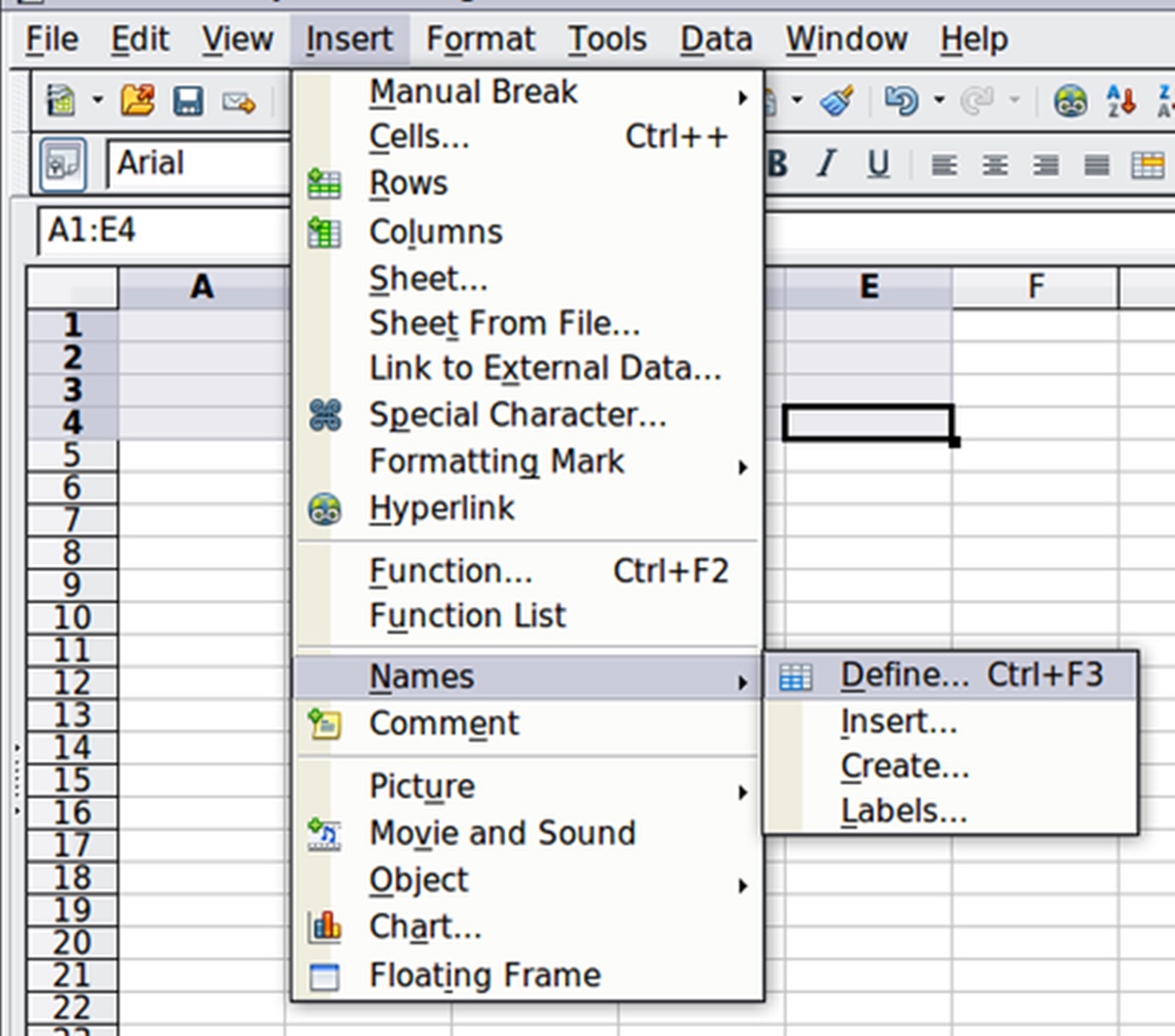
Using Named Ranges

Named ranges in OpenOffice Calc provide a convenient and user-friendly way to refer to specific cells or ranges using custom names instead of cell references. By assigning a name to a range, you can simplify your formulas, enhance readability, and create more maintainable spreadsheets. Using named ranges helps you streamline your calculations and improve the efficiency of working with data.

To create a named range, you can use the Name Box located next to the formula bar. Simply select the range of cells you want to name, type the desired name in the Name Box, and press Enter. You can also define named ranges using the Define Names dialog box.

Once you have assigned a name to a range, you can use that name in place of cell references in formulas throughout your spreadsheet. For example, instead of using the formula =SUM(A1:A10), you can use the named range “Sales” and write =SUM(Sales). This makes your formulas more intuitive and easier to understand.

Named ranges offer several benefits:

Clarity and readability: Named ranges improve the readability of your formulas by using descriptive names instead of cell references. This helps you and other users better understand the purpose of the range in the formula.
Flexibility and maintainability: If you need to change the size or location of a range, you can update the named range in a single place, and all formulas using that name will automatically adjust. This reduces the risk of errors and simplifies spreadsheet maintenance.
Data organization: Named ranges allow you to organize your data more effectively. You can create named ranges for different data categories or subsets, making it easier to navigate and analyze specific parts of your spreadsheet.
Collaboration: Using named ranges promotes collaboration by providing a common language for communicating and referencing data. It helps ensure that everyone understands and uses the correct data ranges consistently across the spreadsheet.

Named ranges can be useful for a variety of scenarios, including calculations, charts, conditional formatting, data validation, and more. Take advantage of named ranges in your OpenOffice Calc spreadsheets to enhance efficiency and create more intuitive and manageable formulas.

Using Data Analysis Tools

OpenOffice Calc provides a range of built-in data analysis tools that allow you to perform complex calculations, generate insights, and visualize your data more effectively. These tools enable you to uncover patterns, identify trends, and make data-driven decisions within your spreadsheets. By leveraging data analysis tools, you can gain valuable insights and extract meaningful information from your data.

Calc offers various data analysis tools, including:

PivotTables: PivotTables allow you to summarize, analyze, and manipulate large datasets quickly. They provide a way to slice and dice data, create custom reports, and perform calculations such as sum, average, count, and more based on different dimensions.
Sorting and Filtering: Calc allows you to sort data based on specific criteria, such as alphabetical order or numerical values. You can also apply filters to display only the data that meets specific conditions, allowing for focused analysis.
Subtotals: Subtotals allow you to group and summarize data based on specific columns. You can calculate subtotals for various categories, perform calculations within each group, and create customized reports.
Data Validation: Data validation helps ensure that the data entered in your spreadsheet meets specific criteria or constraints. It allows you to define rules for acceptable input, control data accuracy, and prevent errors.
What-If Analysis: Calc provides tools for conducting “what-if” analysis, allowing you to explore different scenarios and understand the impact of changing variables. Features like Goal Seek and Scenario Manager help you understand how changes to input values influence outcomes.
Statistical Analysis: Calc offers a range of statistical functions and tools to calculate statistical measures, perform regression analysis, determine correlations, and more. These tools enable you to uncover patterns, gain insights, and analyze data from a statistical perspective.

By utilizing these data analysis tools, you can enhance your ability to manipulate, analyze, and interpret data within your spreadsheets effectively. These tools support critical decision-making processes, enable you to identify patterns and trends, and facilitate a deeper understanding of your data.

Take advantage of the data analysis tools in OpenOffice Calc to perform advanced calculations, generate meaningful reports, and gain valuable insights into your data. These tools empower you to make informed decisions based on robust analysis and aids in effective data-driven solutions.

Troubleshooting Formulas

Working with formulas in OpenOffice Calc can occasionally lead to errors or unexpected results. However, with a systematic approach to troubleshooting, you can easily identify and rectify formula-related issues. Here are some common techniques to troubleshoot formulas:

Check Syntax: Ensure that your formulas have the correct syntax, including balanced parentheses and the correct use of operators and functions. A small typographical error or missing closing parentheses can cause formula errors.
Verify Cell References: Double-check that the cell references in your formulas accurately correspond to the intended cells. Incorrect cell references can result in incorrect calculations or data retrieval.
Examine Error Messages: When a formula produces an error, Calc provides error messages that can help identify the issue. Common error messages include #VALUE!, #REF!, #DIV/0!, #NAME?, and #N/A. Understanding these error messages can assist in troubleshooting.
Trace Precedents and Dependents: Use the Trace Precedents and Trace Dependents tools to analyze how cells are linked to each other. This allows you to identify cells that contribute to formula errors or ensure that formulas are referencing the correct data.
Use Evaluation Tools: Utilize Calc’s built-in formula evaluation tools to step through your formulas and observe the intermediate results at each stage. This can help pinpoint which part of the formula is causing the issue.
Test Formulas: Test parts of your formulas individually to isolate the problematic segment. By doing this, you can identify any errors or issues within specific sections of the formula and troubleshoot them accordingly.
Review Data Types: Ensure that the data types of the values being used in the formula match the expected data types. For example, attempting to perform mathematical operations on text or using non-numeric data in functions that require numbers can result in errors.
Explore Function Documentation: Consult the Calc documentation or online resources to review the syntax and parameters of specific functions. This will help ensure that you are using the functions correctly within your formulas.

By utilizing these troubleshooting techniques, you can efficiently identify and resolve formula errors within your OpenOffice Calc spreadsheets. Troubleshooting formulas is an essential part of creating accurate calculations and understanding the underlying data. With practice, you will become proficient in identifying and rectifying formula-related issues.