How to Use the Excel Subtotal Function

What is the Excel Subtotal Function?

The Excel Subtotal function is a powerful tool that allows users to perform calculations and create summaries for a specified range of data. It is particularly useful when working with large datasets or when conducting data analysis. The Subtotal function can perform various operations, such as sum, average, count, maximum, minimum, and more, depending on the selected function code.

This function is different from other Excel functions because it can perform calculations on both visible and hidden rows in a filtered range. It also provides an option to automatically insert subtotals and grand totals for grouped data without the need for manual calculations.

The Subtotal function is commonly used in conjunction with filtering and grouping functions to analyze data in a more organized and structured manner. It helps users create customized reports, summaries, and subtotals, providing valuable insights into the data.

With the Excel Subtotal function, you can easily perform calculations on subsets of data within a larger dataset, allowing for better analysis and understanding of the information. It saves time and effort by automating calculations and provides flexibility to adjust the calculation method based on the requirements.

As a versatile tool, the Subtotal function is widely used in various industries and fields, including finance, accounting, sales, marketing, human resources, and more. It enables users to effectively manage and analyze data, make informed decisions, and generate meaningful reports.

Syntax of the Subtotal Function

The syntax of the Excel Subtotal function is as follows:

=SUBTOTAL(function_code, range1, [range2], ...)

The function_code argument is a required parameter that specifies the type of calculation to be performed. It is a number between 1 and 11 or between 101 and 111, corresponding to different calculation methods.

For calculation methods including hidden values, use numbers between 1 and 11.
For calculation methods excluding hidden values, use numbers between 101 and 111.

The range1 argument is a required parameter that specifies the range of cells or range names to be included in the calculation.

The range2, range3, … arguments are optional parameters that allow additional ranges to be included in the calculation. You can specify up to 255 ranges.

It’s important to note that the Subtotal function automatically excludes other Subtotal functions within the specified range from the calculation to avoid double-counting.

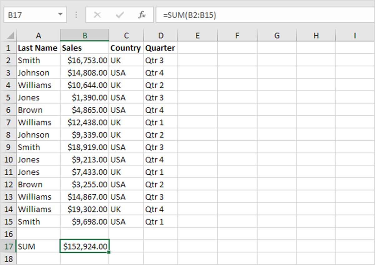
Here’s an example of the Subtotal function:

=SUBTOTAL(9, A2:A10)

This formula calculates the sum of the visible values in cells A2 to A10 using the function code 9, which represents the SUM function.

By using different function codes and ranges, you can perform various calculations, such as averages, counts, maximums, minimums, and more, on different sets of data.

The Subtotal function offers great flexibility and allows you to customize your calculations based on the specific requirements of your data analysis.

How to Use the Subtotal Function

The Subtotal function in Excel is easy to use and offers a wide range of options for calculating and summarizing data. Here are the steps to effectively use the Subtotal function:

Select the Range: Start by selecting the range of cells that you want to include in the calculation. This can be a single column, multiple columns, or a range of cells.
Open the Subtotal Dialog Box: Go to the “Data” tab in the Excel ribbon, then click on the “Subtotal” button in the “Outline” group. This will open the Subtotal dialog box.
Specify the Function: In the Subtotal dialog box, choose the function you want to apply to the selected range. You can select from options such as Sum, Average, Count, Maximum, Minimum, and more. Each function has a corresponding function code that you need to specify.
Select the Summary Columns: Select the columns within the selected range for which you want to display subtotals. You can choose one or multiple columns based on your requirements.
Choose the Location for the Subtotals: Decide whether you want the subtotals to be displayed below each group or at the top of each group. You can also choose to insert page breaks between the groups for better organization.
Apply the Subtotal Function: Click the “OK” button in the Subtotal dialog box to apply the function to the selected range. Excel will automatically insert the subtotals based on the chosen settings.

Once you have applied the Subtotal function, Excel will display the subtotals in the selected columns. It will also group the data based on the specified column(s) and provide options to expand or collapse these groups for better visibility.

By following these steps, you can easily utilize the Subtotal function in Excel to perform calculations and create summaries for your data. It is a powerful tool for analyzing large datasets, generating reports, and gaining valuable insights from your data.

Step 1: Select the Range

The first step in using the Subtotal function in Excel is to select the range of cells that you want to include in the calculation. The range can be a single column, multiple columns, or a range of cells that contains the data you want to analyze and summarize.

To select a range, follow these steps:

Click and drag your mouse over the cells to highlight the desired range. Alternatively, you can click on the first cell in the range, hold down the Shift key, and then click on the last cell in the range.
If your data is in a table format or is organized into named ranges, you can select the entire table or named range by clicking on a cell within the table or named range.
Make sure to include any header rows or columns that are part of the data you want to analyze. Excel will automatically exclude these header rows/columns from the calculations.

By selecting the range accurately, you ensure that the Subtotal function applies the calculation only to the desired data set.

It’s important to note that the Subtotal function works well with filtered data. If you have applied filters to your data, make sure to select only the visible cells within the filtered range. This way, the Subtotal function will perform calculations on the visible data and exclude any hidden or filtered-out rows.

By correctly selecting the range, you set the foundation for performing calculations and generating subtotals using the Subtotal function in Excel. Once the range is selected, you can proceed to the next steps to configure the calculation methods, specify summary columns, and apply the Subtotal function.

Step 2: Open the Subtotal Dialog Box

After selecting the range of cells that you want to include in the calculation, the next step is to open the Subtotal dialog box in Excel. This dialog box provides the necessary options for configuring the Subtotal function and applying it to the selected range.

To open the Subtotal dialog box, follow these steps:

Open Excel and make sure that the workbook containing your data is active.
Go to the “Data” tab in the Excel ribbon at the top of the screen.
In the “Outline” group, click on the “Subtotal” button. It typically looks like a small number 9 inside a blue square.

Clicking on the Subtotal button will open the Subtotal dialog box, where you can specify the function code, select the summary columns, and determine the location of the subtotals.

The Subtotal function in Excel offers a variety of options for calculating and summarizing data. The Subtotal dialog box allows you to customize the calculation based on your specific requirements.

Once the Subtotal dialog box is open, you can proceed to the next step of specifying the function code. This function code determines the type of calculation that will be applied to the selected range.

By opening the Subtotal dialog box, you gain access to the configuration options for the Subtotal function. It is an essential step in utilizing the Subtotal function effectively and accurately summarizing your data in Excel.

Step 3: Specify the Function

After opening the Subtotal dialog box in Excel, the next step is to specify the function code that corresponds to the type of calculation you want to perform on the selected range. The function code determines the specific operation that the Subtotal function will apply.

To specify the function code, follow these steps:

In the Subtotal dialog box, you will see a list of available functions from which you can choose.
Select the function that best suits your analysis requirements. Some commonly used function codes include:
- 1: SUM – adds up the values in the selected range
- 2: AVERAGE – calculates the average of the values in the selected range
- 3: COUNT – counts the number of cells that contain values in the selected range
- 4: MAX – determines the maximum value in the selected range
- 5: MIN – identifies the minimum value in the selected range
- 9: SUM – adds up only the visible values in the selected range (when using filtered data)
- There are additional function codes available, offering a range of options for calculations.
Once you have selected the function code, click on the “OK” button to confirm your choice.

After specifying the function code, Excel will apply the selected function to the range of cells you have chosen. The Subtotal function will then perform the desired calculation on the selected data and generate the appropriate subtotals.

By specifying the function code accurately, you can ensure that the Subtotal function provides the desired calculation result for your data analysis. It allows you to tailor the Subtotal function to your specific needs and obtain the desired insights into your data.

Step 4: Select the Summary Columns

Once you have specified the function code in the Subtotal dialog box, the next step is to select the summary columns. These are the columns within the selected range for which you want to display the subtotals.

To select the summary columns, follow these steps:

In the Subtotal dialog box, you will see a list of columns based on the range you have selected.
Check the box next to each column for which you want to display subtotals.
If you want to display subtotals for all columns, you can click the “At each change in” checkbox at the bottom of the dialog box. This will automatically select all columns for subtotals.
You can also select multiple non-adjacent columns by holding down the “Ctrl” key and clicking on the desired column headers.

By selecting the summary columns, you tell Excel which columns you want to include in the calculation and display subtotals for. This allows you to focus on specific data points and gain insights into the summarized information.

It’s important to note that selecting the appropriate summary columns depends on the analysis you want to perform and the insights you’re seeking. Consider the key columns that provide meaningful information and contribute to the overall analysis when making your selections.

By choosing the summary columns effectively, you can generate comprehensive subtotals for the selected range, highlighting the relevant data points and aiding in your data analysis process.

Step 5: Choose the Location for the Subtotals

After selecting the summary columns in the Subtotal dialog box, the next step is to choose the location for the subtotals. This determines where the subtotals will be displayed in relation to the grouped data.

To choose the location for the subtotals, follow these steps:

In the Subtotal dialog box, you will find two options for the location of the subtotals: “Summary below data” and “Summary above data“.
Select either of these options based on your preference and the visual presentation of your data.
If you choose the “Summary below data” option, Excel will insert a row with the subtotal values below each group of data.
If you choose the “Summary above data” option, Excel will insert a row with the subtotal values above each group of data.
Additionally, you can check the “Page break between groups” checkbox if you want Excel to insert page breaks between each group, providing better organization in your report or worksheet.

Choosing the location for the subtotals is a matter of personal preference and the desired presentation of your summarized data. It helps in organizing and displaying the subtotals in a way that is visually appealing and enhances the understandability of the information.

Consider your intended audience and the purpose of the analysis when selecting the location for the subtotals. Depending on the context, you may choose to display the subtotals below or above the grouped data to optimize clarity and readability.

By customizing the location of the subtotals, you create a structured and visually appealing presentation of your summarized data, facilitating a better understanding of the important information within your Excel worksheet or report.

Step 6: Apply the Subtotal Function

After configuring the Subtotal function settings, the final step is to apply the function to the selected range. This will generate the desired subtotals based on the specified calculations and display them in the chosen location.

To apply the Subtotal function, follow these steps:

Ensure that the Subtotal dialog box is still open.
Click on the “OK” button located at the bottom of the dialog box.

Once you click “OK”, Excel will immediately apply the Subtotal function to the selected range. It will calculate the subtotals based on the specified function code and display them in the chosen location, either above or below the grouped data.

The subtotals will be inserted into the worksheet as additional rows, with the summary calculations based on the chosen function applied to the selected summary columns.

At this point, you will be able to see the subtotals displayed in the designated location, providing a condensed summary of the data within each group.

It’s important to note that if you make any changes to the data or add new rows within the selected range, you may need to reapply the Subtotal function to update the subtotals dynamically.

By applying the Subtotal function, you can efficiently analyze and summarize your data in Excel, generating valuable insights and making it easier to interpret your information effectively.

Understanding the Different Subtotal Functions

The Subtotal function in Excel offers a variety of calculation options to suit different analytical needs. Each function code represents a specific calculation method that can be applied to the selected range. Understanding the different Subtotal functions allows you to choose the most appropriate one for your data analysis. Here are some of the commonly used Subtotal functions:

Function Code 1 (SUM): This function calculates the sum of the values in the selected range. It provides the total sum of all the numbers in the chosen summary columns.
Function Code 2 (AVERAGE): This function calculates the average of the values in the selected range. It gives you the average value for each summary column.
Function Code 3 (COUNT): This function counts the number of cells in the selected range that contain values. It provides a count of the data points in each summary column.
Function Code 4 (MAX): This function identifies the maximum value in the selected range. It gives you the highest value in each summary column.
Function Code 5 (MIN): This function determines the minimum value in the selected range. It provides the lowest value in each summary column.
Function Code 9 (SUM – Visible Only): This function calculates the sum of only the visible values in the selected range. It excludes hidden or filtered-out rows, making it useful when working with filtered data.

These are just a few examples of the Subtotal functions available in Excel. There are additional function codes, ranging from 1 to 11 and 101 to 111, that offer different calculation methods.

Understanding the different Subtotal functions allows you to choose the most appropriate calculation for your specific analysis requirements. By selecting the right Subtotal function, you can generate meaningful summaries and extract valuable insights from your data set.

Applying Multiple Subtotal Functions to the Same Range

In Excel, it is possible to apply multiple Subtotal functions to the same range of data. This allows you to perform multiple calculations simultaneously and generate comprehensive summaries. By applying multiple Subtotal functions, you can gain deeper insights and analyze your data from different perspectives.

To apply multiple Subtotal functions to the same range, follow these steps:

First, select the range of data that you want to include in the calculations.
Next, open the Subtotal dialog box by going to the “Data” tab and clicking on the “Subtotal” button in the “Outline” group.
In the Subtotal dialog box, specify the first Subtotal function by selecting the function code and summary columns.
Click on the “OK” button to apply the first Subtotal function.
Repeat the process to add additional Subtotal functions. Each time you open the Subtotal dialog box, select a new function code and summary columns.
Click on the “OK” button after configuring each Subtotal function.

By following these steps, you can apply multiple Subtotal functions to the same range. Excel will perform each calculation separately and display the corresponding subtotals in the specified location.

Applying multiple Subtotal functions allows you to generate a comprehensive analysis of your data, showcasing different aspects and calculations. For example, you can determine the sum, average, count, and other statistics for different columns all at once.

It’s important to note that when applying multiple Subtotal functions, you may want to carefully select the summary columns to avoid overlapping or redundant calculations. Consider your analysis goals and the specific insights you want to derive from your data when choosing the Subtotal functions and summary columns.

By applying multiple Subtotal functions to the same range, you can enhance your data analysis capabilities and gain a more nuanced understanding of your data set. It allows for a comprehensive summary that encompasses multiple calculations and provides valuable insights for informed decision-making.

Removing Subtotals from a Range

In Excel, if you have applied subtotals to a range of data using the Subtotal function, you may later decide to remove those subtotals. Removing subtotals can be necessary when the data changes or when you want to revert to the original view of your data without the summary calculations.

To remove subtotals from a range in Excel, follow these steps:

Select the range that contains the subtotals.
Go to the “Data” tab in the Excel ribbon.
In the “Outline” group, click on the “Subtotal” button.
In the Subtotal dialog box, ensure that the “Remove All” option is selected.
Click on the “OK” button.

By following these steps, Excel will remove all subtotals from the selected range, restoring the original view of the data without any summary calculations.

It’s important to note that when you remove subtotals, any grouping or outlining effects that were automatically applied may also be removed. Therefore, if you want to preserve any existing grouping or outlining, it’s recommended to use the “Remove All” option with caution.

Removing subtotals allows you to clean up your data and restore it to its original form, eliminating any calculations or summary information that may have been added using the Subtotal function. This gives you more flexibility in terms of data manipulation and analysis.

Whether your data has changed, or you simply don’t need the subtotals anymore, being able to easily remove them from a range can help maintain the integrity and accuracy of your data in Excel.

Using the Subtotal Function with AutoFilter

The Subtotal function in Excel is compatible with the AutoFilter feature, which allows you to filter your data based on specific criteria. By combining the Subtotal function with AutoFilter, you can perform calculations and generate subtotals on filtered data, giving you more flexibility and control over your analysis.

To use the Subtotal function with AutoFilter, follow these steps:

Select the range of data that you want to include in the calculations.
Apply the AutoFilter by going to the “Data” tab and clicking on the “Filter” button.
In the filtered range, open the Subtotal dialog box by going to the “Data” tab and clicking on the “Subtotal” button in the “Outline” group.
Specify the function code and summary columns for the Subtotal function.
Choose the desired location for the subtotals, either below or above the grouped data.
Click on the “OK” button to apply the Subtotal function.

By following these steps, Excel will calculate the subtotals based on the specified function and display them in the chosen location, considering only the visible data as per the applied AutoFilter.

The Subtotal function with AutoFilter is particularly useful when you want to analyze specific subsets of your data. It allows you to focus on filtered portions of your data and obtain relevant subtotals based on those filtered records.

It’s important to note that when using the Subtotal function with AutoFilter, you may need to update the subtotals if any changes are made to the filter criteria or if new data is added. To do this, simply reapply the Subtotal function after adjusting the AutoFilter as needed.

By leveraging the power of the Subtotal function in combination with AutoFilter, you can perform calculations and generate subtotals on filtered data, resulting in more targeted and insightful data analysis in Excel.

Benefits of Using the Subtotal Function

The Subtotal function in Excel offers several benefits that can greatly enhance your data analysis and reporting capabilities. Here are some key benefits of using the Subtotal function:

Data summarization: The Subtotal function allows you to summarize large datasets by performing various calculations, such as sum, average, count, maximum, minimum, and more. It provides concise and meaningful summaries, making it easier to understand and interpret complex data.
Grouping and organization: With the Subtotal function, you can easily group and organize your data based on specific criteria. This allows you to create hierarchical views and analyze subsets of data within a larger dataset, providing a more structured and organized representation of your information.
Dynamic calculations: The Subtotal function dynamically recalculates the subtotals and summaries as you make changes to your data. This saves you time and effort, as you don’t need to manually update your calculations whenever the underlying data changes.
Visibility customization: You have the flexibility to choose where to display the subtotals, either above or below the grouped data. This gives you control over the visual presentation of your summaries and allows you to tailor the view to meet your specific requirements.
Compatible with AutoFilter: The Subtotal function works seamlessly with Excel’s AutoFilter feature. This means you can perform calculations and generate subtotals on filtered data, allowing for more targeted analysis and customized views of your data.
Integration with other Excel functions: The Subtotal function can be combined with other Excel functions, such as IF, SUMIF, COUNTIF, etc. This enables you to perform advanced calculations and apply specific conditions to your subtotals, making your analysis more robust and insightful.

Overall, the Subtotal function offers a range of benefits that streamline data summarization, enhance data organization, and simplify analysis. It helps you make sense of your data, draw valuable insights, and present your findings in a clear and concise manner.

Limitations of the Subtotal Function

While the Subtotal function in Excel is a powerful tool for data analysis, it also has some limitations that are important to be aware of. Understanding these limitations can help you use the Subtotal function effectively and avoid potential issues. Here are some key limitations of the Subtotal function:

Single-level grouping: The Subtotal function supports single-level grouping, meaning it can only handle one level of grouping at a time. If you need to perform calculations on multiple levels of grouping, you may need to resort to more advanced techniques, such as Pivot Tables.
No custom calculations: The predefined calculations offered by the Subtotal function may not cover all your specific requirements. If you need to perform custom calculations or apply complex formulas to your data, you may need to explore other Excel functions or tools.
No support for merged cells: If your data contains merged cells within the range you want to apply the Subtotal function to, it may lead to unexpected results or errors. It’s best to avoid using merged cells when working with the Subtotal function.
No support for non-numeric data: The Subtotal function is primarily designed for numeric data, and it may not produce meaningful results when applied to non-numeric columns. Ensure that the columns you choose for subtotals contain appropriate data types.
Limited customization options: While the Subtotal function provides some customization options, such as choosing the location of subtotals, it may not offer the level of customization or formatting options you desire. You may need to perform additional formatting or customization manually to achieve your desired output.
Data must be sorted correctly: The Subtotal function assumes your data is correctly sorted based on the grouping column(s). If your data is not sorted correctly, the resulting subtotals may not be accurate. Ensure that your data is sorted correctly before applying the Subtotal function.

It’s important to consider these limitations and evaluate whether the Subtotal function is the most suitable tool for your specific data analysis needs. If the limitations pose significant challenges or constraints, you may need to explore alternative methods or functions in Excel to achieve your desired results.