How to Use Excel's AutoFormat Feature

What is AutoFormat in Excel?

AutoFormat is a powerful feature in Microsoft Excel that allows you to quickly apply pre-designed formatting styles to a range of cells, making your data visually appealing and easier to understand. It saves you time and effort by automatically formatting your data based on predefined templates, eliminating the need for manual formatting.

With the AutoFormat feature, you can instantly change the font, cell border, fill color, and other formatting elements of your selected cells. This feature is especially useful when dealing with large datasets or when you want to give your spreadsheet a professional look without spending hours on manual formatting.

Excel offers a wide range of AutoFormat templates, including styles for tables, headings, data bars, and conditional formatting. Each template is designed to enhance the readability and presentation of your data, ensuring that important information stands out and catches the reader’s attention.

Whether you are creating reports, analyzing financial data, or organizing your personal budget, the AutoFormat feature in Excel can help you transform your data into clear and visually appealing presentations. It allows you to focus on the content and analysis while Excel takes care of the formatting details.

Now that you understand the basic concept of AutoFormat in Excel, let’s explore how you can access and use this feature to improve your spreadsheet formatting effortlessly.

How to Access the AutoFormat Feature

Accessing the AutoFormat feature in Excel is straightforward, and there are multiple ways to do it:

Using the Ribbon Menu: The Ribbon is Excel’s main toolbar, and it provides easy access to various features and commands. To use AutoFormat via the Ribbon, follow these steps:
a. Select the range of cells that you want to apply formatting to.
b. Go to the “Home” tab on the Ribbon.
c. In the “Styles” group, click on the “Format as Table” button.
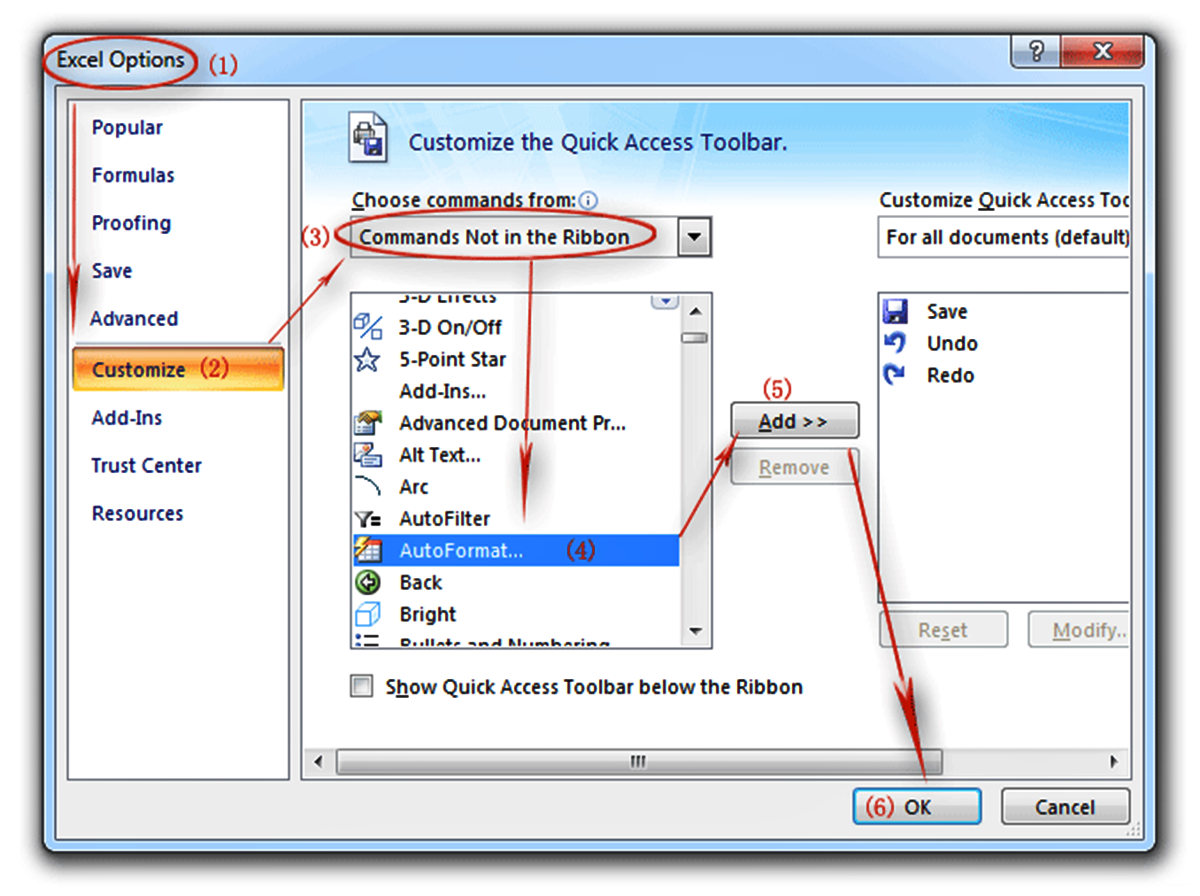
d. Choose the desired table style from the available options.

Using the Quick Access Toolbar: The Quick Access Toolbar is a customizable toolbar located right above the Ribbon. You can add frequently used commands to this toolbar for quick access. To use AutoFormat via the Quick Access Toolbar:
a. Select the range of cells that you want to format.
b. Click on the downward arrow on the Quick Access Toolbar.
c. From the drop-down menu, select “Format as Table”.
d. Choose the desired table style from the available options.

Using the Format Options menu: Another way to access AutoFormat is through the Format Options menu:
a. Select the range of cells you wish to format.
b. Right-click on the selected cells to open the context menu.
c. From the menu, choose “Format Cells”.
d. In the Format Cells dialog box, navigate to the “Table” tab and select the desired table style.

These methods allow you to access the AutoFormat feature quickly and conveniently. Once you have accessed AutoFormat, you can proceed to apply the desired formatting style to your selected cells.

Applying AutoFormat to a Range of Cells

Once you have accessed the AutoFormat feature in Excel, applying it to a range of cells is a breeze. Here’s how you can do it:

Select the Cells: Choose the range of cells to which you want to apply the AutoFormat. It can be a continuous range or multiple non-contiguous cells.

Access the AutoFormat Options: Depending on the method you used to access AutoFormat, you will either see a gallery of pre-designed table styles or a dialog box with formatting options.

Choose a Format Style: Browse through the available table styles or formatting options and select the one that best suits your data needs. You can hover over each style to preview how it will look on your selected cells.

Apply the Format: Once you have selected a table style or formatting option, click on it to apply it to the selected cells. Excel will automatically format the cells according to the chosen style.

After applying the AutoFormat, your selected cells will be instantly formatted based on the chosen style. The font, cell borders, fill colors, and other formatting elements will be applied to make your data visually appealing and easier to understand.

Keep in mind that the AutoFormat feature is not limited to tables; you can also use it to format other elements such as headings, data bars, and conditional formatting. Excel provides various options for customizing and enhancing the appearance of your data.

Now that you know how to apply AutoFormat to a range of cells, you can experiment with different styles and formatting options to make your spreadsheets more visually appealing and professional.

Customizing AutoFormat Options

Excel’s AutoFormat feature provides pre-designed table styles and formatting options, but you also have the flexibility to customize these options to suit your specific needs. Here’s how you can customize AutoFormat in Excel:

Access AutoFormat Options: Depending on the method you used to access AutoFormat, you may have different options for customization. Look for an “Options” or “Customize” button that allows you to modify the AutoFormat settings.

Modify Font and Formatting: In the AutoFormat options, you can adjust the font style, size, and color used for different elements of the table. You can also modify cell borders, fill colors, and other formatting aspects to create a unique style that aligns with your document’s theme or personal preference.

Save Custom Format: Once you have customized the AutoFormat options to your liking, you can save your custom format as a new style. This allows you to apply the same formatting to other tables or ranges in the future without having to recreate the customization each time.

Modify Existing Formats: If you want to make changes to an existing AutoFormat style, you can access the Format Styles Manager or a similar option to edit the predefined styles. This way, you can fine-tune the default styles to meet your specific requirements.

Apply Conditional Formatting: AutoFormat can also be combined with Excel’s powerful conditional formatting feature. This allows you to set rules based on cell values or other criteria and apply specific formatting automatically. By customizing the conditional formatting rules, you can further tailor the appearance of your data to highlight important information or identify specific trends.

By customizing AutoFormat options, you can create a unique and consistent formatting style that matches your preferences and requirements. Whether you prefer a clean and minimalist look or a bold and vibrant design, Excel provides the flexibility to customize the formatting to your liking.

Next, we’ll explore how to remove AutoFormat from a range of cells, in case you want to revert to the default formatting or apply a different style.

Removing AutoFormat from a Range of Cells

If you have applied AutoFormat to a range of cells in Excel, but later decide you want to remove it, you can easily revert to the default formatting or apply a different style. Here’s how you can remove AutoFormat from a range of cells:

Select the Formatted Cells: Identify the range of cells that have the AutoFormat applied. You can click on any cell within that range to select it, and then press Ctrl+Shift+Spacebar to select the entire range. Alternatively, you can click and drag over the range to select it manually.

Access the Clear Formatting Option: Once you have selected the formatted cells, go to the “Home” tab on the Ribbon. In the “Editing” group, you will find the “Clear” button. Click on the drop-down arrow next to it and select “Clear Formats” from the available options. This will remove the AutoFormat and revert the selected cells to the default formatting.

Apply a Different Format: If you want to remove AutoFormat and apply a different formatting style, you can do so by selecting the cells again and accessing the AutoFormat feature. Choose a new format option or custom style, and Excel will apply it to the selected cells while removing the previous AutoFormat.

By following these steps, you can easily remove AutoFormat from a range of cells in Excel. Whether you want to revert to the default formatting or apply a different style, Excel provides the tools to make the necessary changes quickly and efficiently.

Next, let’s explore how you can combine AutoFormat with conditional formatting to further enhance the visual presentation of your data.

Using AutoFormat with Conditional Formatting

Excel allows you to combine the powerful AutoFormat feature with conditional formatting to create dynamic and visually appealing spreadsheets. By applying conditional formatting rules along with AutoFormat, you can highlight specific data points or trends based on predefined criteria. Here’s how you can use AutoFormat with conditional formatting:

Select the Range for Conditional Formatting: Identify the range of cells that you want to format based on specific conditions. This can be a single column, a row, or even the entire worksheet.

Access the Conditional Formatting Options: Go to the “Home” tab on the Ribbon and click on the “Conditional Formatting” button in the “Styles” group. From the drop-down menu, choose the desired conditional formatting rule or click on “New Rule” to create a custom rule.

Set the Formatting Criteria: In the Conditional Formatting dialog box, specify the conditions that should be met for the formatting to be applied. This can include comparisons with other values, the use of formulas, or other criteria based on your specific data requirements.

Choose the Formatting Style: After defining the conditions, select the formatting style that you want to apply when the conditions are met. You can choose a predefined format or customize your own style using font, fill colors, cell borders, and other formatting options.

Apply AutoFormat: Once you have set up the conditional formatting rule, you can enhance the formatting even further by applying AutoFormat. Access the AutoFormat feature and select a table style or format option that complements the conditional formatting. This will give your data an additional layer of visual organization.

Using AutoFormat with conditional formatting allows you to present your data in a more meaningful and impactful way. By highlighting specific values or trends, you can draw attention to important information and make it easier for others to interpret the data.

Now that you know how to use AutoFormat with conditional formatting, let’s explore some tips and tricks for getting the most out of this feature.

Tips and Tricks for Using AutoFormat in Excel

Excel’s AutoFormat feature can be a valuable tool for enhancing the visual appeal and organization of your spreadsheets. To make the most out of AutoFormat, here are some helpful tips and tricks:

Preview Before Applying: Excel allows you to preview different AutoFormat styles before applying them. Take advantage of this feature to see how the formatting will look on your selected cells and choose the style that best suits your data.

Save Custom Formats: If you have customized the AutoFormat options to create a unique formatting style, consider saving it as a custom format. This way, you can easily apply the same formatting to other tables or ranges in the future without having to recreate the customization each time.

Combine with Conditional Formatting: Experiment with combining AutoFormat with Excel’s conditional formatting feature. By using both features together, you can create visually appealing spreadsheets while highlighting specific data based on conditions or criteria.

Explore Table Styles: AutoFormat provides a variety of table styles that you can apply to your data. Take the time to explore and experiment with different table styles to find the one that best represents your information and enhances its readability.

Apply Consistently: To maintain a professional and consistent appearance throughout your spreadsheet, apply AutoFormat consistently. Use the same format style for tables or related data ranges to create a cohesive look that is easy to navigate.

By implementing these tips and tricks, you can utilize the AutoFormat feature in Excel to create visually appealing and well-organized spreadsheets. Remember to consider the specific needs of your data and audience to choose the formatting options that best enhance its readability and presentation.

Next, let’s explore some examples of how AutoFormat can be used in different scenarios to transform your data visually.

Examples of Using AutoFormat in Excel

AutoFormat in Excel offers a wide range of possibilities for transforming and enhancing your data presentation. Here are a few examples of how you can utilize AutoFormat in different scenarios:

Financial Reports: When creating financial reports, you can use AutoFormat to quickly format tables with monetary values. Apply a table style that includes currency symbols and formats numbers with appropriate decimal places, making your financial data more readable and professional.

Sales and Marketing Analysis: AutoFormat can be utilized to visually represent sales data, marketing metrics, or campaign performance. Apply colorful table styles and use conditional formatting to highlight key figures, such as high sales volumes or low conversion rates, making it easier to identify trends and insights.

Project Management: Use AutoFormat to organize project-related data, such as task lists, timelines, or resource allocation tables. Apply a table format that separates headers from data rows, and use conditional formatting to highlight urgent or overdue tasks for better project visibility and tracking.

Survey Results: AutoFormat can be useful in formatting survey or questionnaire results. Apply a table style that differentiates question headers from respondents’ answers. Use conditional formatting to highlight specific responses, such as satisfaction ratings, to quickly identify areas that need attention or improvement.

Personal Budgeting: AutoFormat can be applied to formatting personal budget spreadsheets. Use a table style with clear headings and apply conditional formatting to highlight expenses exceeding the allocated budget. This makes it easier to track and analyze your spending patterns.

These examples illustrate how AutoFormat can be used for different purposes and industries. By selecting the appropriate table styles and applying conditional formatting rules, you can transform your raw data into visually striking and informative presentations.

Now that you have a good understanding of how to use AutoFormat in Excel, you can apply these concepts to your own projects and make your data presentation more professional and engaging.

Final Thoughts on Excel’s AutoFormat Feature

Excel’s AutoFormat feature is a valuable tool that simplifies and accelerates the process of formatting data in spreadsheets. It allows users to apply pre-designed table styles and formatting options to ranges of cells, making data more visually appealing and easier to understand.

By utilizing AutoFormat, you can save time and effort that would otherwise be spent on manual formatting. The feature provides a wide range of formatting templates suitable for various types of data, including financial reports, sales analyses, project management tables, survey results, and personal budgets.

Customization options within AutoFormat enable users to modify font styles, colors, cell borders, and other elements to create a unique and consistent formatting style. Additionally, AutoFormat can be combined with Excel’s conditional formatting to highlight specific data points based on predefined criteria, further enhancing the visual presentation of information.

Using AutoFormat not only improves the aesthetics of your spreadsheets but also makes your data more accessible and comprehensible to others. It allows you to present information in a structured and organized manner, helping readers quickly identify key figures, trends, and insights.

Remember to preview different AutoFormat styles before applying them and save any custom formats you create for future use. Consistent application of AutoFormat throughout your spreadsheet ensures a professional and cohesive appearance that enhances the overall user experience.

Whether you are a financial analyst, project manager, survey researcher, or anyone working with data, Excel’s AutoFormat feature is a powerful ally that can significantly enhance your productivity and the visual impact of your work.

Now that you have an understanding of the capabilities and benefits of AutoFormat, it’s time to unleash its potential and transform your spreadsheets into visually appealing and professional presentations of data.